Methods of determining_safety_integrity_level

Methods of Determining Safety Integrity Level.doc Page 1 of 16 14 April 2004
Methods of Determining Safety Integrity Level (SIL)
Requirements - Pros and Cons
by W G Gulland (4-sight Consulting)
1 Introduction
The concept of safety integrity levels (SILs) was introduced during the development of BS
EN 61508 (BSI 2002) as a measure of the quality or dependability of a system which has a
safety function – a measure of the confidence with which the system can be expected to
perform that function. It is also used in BS IEC 61511(BSI 2003), the process sector specific
application of BS EN 61508.
This paper discusses the application of 2 popular methods of determining SIL requirements
– risk graph methods and layer of protection analysis (LOPA) – to process industry
installations. It identifies some of the advantages of both methods, but also outlines some
limitations, particularly of the risk graph method. It suggests criteria for identifying the
situations where the use of these methods is appropriate.
2 Definitions of SILs
The standards recognise that safety functions can be required to operate in quite different
ways. In particular they recognise that many such functions are only called upon at a low
frequency / have a low demand rate. Consider a car; examples of such functions are:
• Anti-lock braking (ABS). (It depends on the driver, of course!).
• Secondary restraint system (SRS) (air bags).
On the other hand there are functions which are in frequent or continuous use; examples of
such functions are:
• Normal braking
• Steering
The fundamental question is how frequently will failures of either type of function lead to
accidents. The answer is different for the 2 types:
• For functions with a low demand rate, the accident rate is a combination of 2 parameters
– i) the frequency of demands, and ii) the probability the function fails on demand (PFD).
In this case, therefore, the appropriate measure of performance of the function is PFD, or
its reciprocal, Risk Reduction Factor (RRF).
• For functions which have a high demand rate or operate continuously, the accident rate
is the failure rate, λ, which is the appropriate measure of performance. An alternative
measure is mean time to failure (MTTF) of the function. Provided failures are
exponentially distributed, MTTF is the reciprocal of λ.
These performance measures are, of course, related. At its simplest, provided the function
can be proof-tested at a frequency which is greater than the demand rate, the relationship
can be expressed as:
PFD = λT/2 or = T/(2 x MTTF), or
RRF = 2/(λT) or = (2 x MTTF)/T

where T is the proof-test interval. (Note that to significantly reduce the accident rate below
the failure rate of the function, the test frequency, 1/T, should be at least 2 and preferably ≥ 5
times the demand frequency.) They are, however, different quantities. PFD is a probability
– dimensionless; λ is a rate – dimension t-1
. The standards, however, use the same term –
SIL – for both these measures, with the following definitions:
Table 1 - Definitions of SILs for Low Demand Mode from BS EN 61508
SIL Range of
Average PFD
Range of RRF1
4 10-5
≤ PFD < 10-4
100,000 ≥ RRF >
10,000
3 10-4
≤ PFD < 10-3
10,000 ≥ RRF >
1,000
2 10-3
≤ PFD < 10-2
1,000 ≥ RRF > 100
1 10-2
≤ PFD < 10-1
100 ≥ RRF > 10
Table 2 - Definitions of SILs for High Demand / Continuous Mode
from BS EN 61508
SIL Range of λ (failures
per hour)
~ Range of MTTF
(years)2
4 10-9
≤ λ < 10-8
100,000 ≥ MTTF >
10,000
3 10-8
≤ λ < 10-7
10,000 ≥ MTTF >
1,000
2 10-7
≤ λ < 10-6
1,000 ≥ MTTF > 100
1 10-6
≤ λ < 10-5
100 ≥ MTTF > 10
In low demand mode, SIL is a proxy for PFD; in high demand / continuous mode, SIL is a
proxy for failure rate. (The boundary between low demand mode and high demand mode is
in essence set in the standards at one demand per year. This is consistent with proof-test
intervals of 3 to 6 months, which in many cases will be the shortest feasible interval.)
Now consider a function which protects against 2 different hazards, one of which occurs at a
rate of 1 every 2 weeks, or 25 times per year, i.e. a high demand rate, and the other at a rate
of 1 in 10 years, i.e. a low demand rate. If the MTTF of the function is 50 years, it would
qualify as achieving SIL1 for the high demand rate hazard. The high demands effectively
proof-test the function against the low demand rate hazard. All else being equal, the
effective SIL for the second hazard is given by:
PFD = 0.04/(2 x 50) = 4 x 10-4
≡ SIL3
So what is the SIL achieved by the function? Clearly it is not unique, but depends on the
hazard and in particular whether the demand rate for the hazard implies low or high demand
mode.
In the first case, the achievable SIL is intrinsic to the equipment; in the second case,
although the intrinsic quality of the equipment is important, the achievable SIL is also
affected by the testing regime. This is important in the process industry sector, where
achievable SILs are liable to be dominated by the reliability of field equipment – process
measurement instruments and, particularly, final elements such as shutdown valves – which
need to be regularly tested to achieve required SILs.
1
This column is not part of the standards, but RRF is often a more tractable parameter than PFD.
2
This column is not part of the standards, but the author has found these approximate MTTF values to be useful
in the process industry sector, where time tends to be measured in years rather than hours.

The differences between these definitions may be well understood by those who are dealing
with the standards day-by-day, but are potentially confusing to those who only use them
intermittently.
3 Some Methods of Determining SIL Requirements
BS EN 61508 offers 3 methods of determining SIL requirements:
• Quantitative method.
• Risk graph, described in the standard as a qualitative method.
• Hazardous event severity matrix, also described as a qualitative method.
BS IEC 61511 offers:
• Semi-quantitative method.
• Safety layer matrix method, described as a semi-qualitative method.
• Calibrated risk graph, described in the standard as a semi-qualitative method, but by
some practitioners as a semi-quantitative method.
• Risk graph, described as a qualitative method.
• Layer of protection analysis (LOPA). (Although the standard does not assign this
method a position on the qualitative / quantitative scale, it is weighted toward the
quantitative end.)
Risk graphs and LOPA are popular methods for determining SIL requirements, particularly in
the process industry sector. Their advantages and disadvantages and range of applicability
are the main topic of this paper.
4 Risk Graph Methods
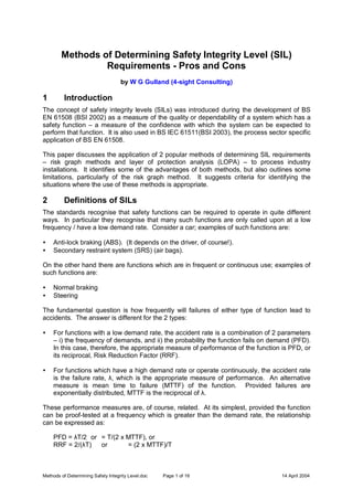
Risk graph methods are widely used for reasons outlined below. A typical risk graph is
shown in Figure 1.
Starting point
for risk reduction
estimation
CA
CB
CC
CD
FA
FB
FA
FB
PA
PB
PA
PB
PA
PB
PA
PB
C = Consequence parameter
F = Frequency and exposure time parameter
P = Possibility of avoiding hazard
W = Demand rate assuming no protection
FA
FB
a
1
2
3
4
b
---
a
1
2
3
4
---
---
a
1
2
3
W3 W2 W1
--- = No safety requirements
a = No special safety requirements
b = A single E/E/PES is not sufficient
1, 2, 3, 4 = Safety Integrity Level
Figure 1 - Typical Risk Graph
The parameters of the risk graph can be given qualitative descriptions, e.g.:
CC ≡ death of several persons.

or quantitative descriptions, e.g.:
CC ≡ probable fatalities per event in range 0.1 to 1.0.
Table 3 - Typical Definitions of Risk Graph Parameters
Consequence
CA Minor injury
CB 0.01 to 0.1 probable fatalities per event
CC > 0.1 to 1.0 probable fatalities per event
CD > 1 probable fatalities per event
Exposure
FA < 10% of time
FB ≥ 10% of time
Avoidability / Unavoidability
PA > 90% probability
of avoiding
hazard
< 10% probability
hazard cannot be
avoided
PB ≤ 90% probability
of avoiding
hazard
≥ 10% probability
hazard cannot be
avoided
Demand Rate
W1 < 1 in 30 years
W2 1 in > 3 to 30 years
W3 1 in > 0.3 to 3 years
The first definition begs the question “What does several mean?” In practice it is likely to be
very difficult to assess SIL requirements unless there is a set of agreed definitions of the
parameter values, almost inevitably in terms of quantitative ranges. These may or may not
have been calibrated against the assessing organisation’s risk criteria, but the method then
becomes semi-quantitative (or is it semi-qualitative? It is certainly somewhere between the
extremities of the qualitative / quantitative scale.)
Table 3 shows a typical set of definitions.
4.1 Benefits
Risk graph methods have the following advantages:
• They are semi-qualitative / semi-quantitative.
§ Precise hazard rates, consequences, and values for the other parameters of the
method, are not required.
§ No specialist calculations or complex modelling is required.
§ They can be applied by people with a good “feel” for the application domain.
• They are normally applied as a team exercise, similar to HAZOP.
§ Individual bias can be avoided.
§ Understanding about hazards and risks is disseminated among team members (e.g.
from design, operations, and maintenance).
§ Issues are flushed out which may not be apparent to an individual.
§ Planning and discipline are required.
• They do not require a detailed study of relatively minor hazards.
§ They can be used to assess many hazards relatively quickly.
§ They are useful as screening tools to identify:
- hazards which need more detailed assessment
- minor hazards which do not need additional protection

so that capital and maintenance expenditures can be targeted where they are most
effective, and lifecycle costs can be optimised.
4.2 The Problem of Range of Residual Risk
Consider the example: CC, FB, PB, W2 indicates a requirement for SIL3.
CC ≡ > 0.1 to 1 probable fatalities per event
FB ≡ ≥ 10% to 100% exposure
PB ≡ ≥ 10% to 100% probability that the hazard cannot be avoided
W2 ≡ 1 demand in > 3 to 30 years
SIL3 ≡ 10,000 ≥ RRF > 1,000
If all the parameters are at the geometric mean of their ranges:
Consequence = √(0.1 x 1.0) probable fatalities per event
= 0.32 probable fatalities per event
Exposure = √(10% x 100%) = 32%
Unavoidability = √(10% x 100%) = 32%
Demand rate = 1 in √(3 x 30) years
= 1 in ~10 years
RRF = √(1,000 x 10,000) = 3,200
(Note that geometric means are used because the scales of the risk graph parameters are
essentially logarithmic.)
For the unprotected hazard:
Worst case risk = (1 x 100% x 100%) / 3 fatalities per year
= 1 fatality in ~3 years
Geometric mean risk = (0.32 x 32% x 32%) / 10 fatalities per year
= 1 fatality in ~300 years
Best case risk = (0.1 x 10% x 10%) / 30 fatalities per year
= 1 fatality in ~30,000 years
i.e. the unprotected risk has a range of 4 orders of magnitude.
With SIL3 protection:
Worst case residual risk = 1 fatality in (~3 x 1,000) years
= 1 fatality in ~3,000 years
Geometric mean residual risk = 1 fatality in (~300 x 3,200) years
= 1 fatality in ~1 million years
Best case residual risk = 1 fatality in (~30,000 x 10,000) years
= 1 fatality in ~300 million years
i.e. the residual risk with protection has a range of 5 orders of magnitude.
Figure 2 shows the principle, based on the mean case.

Partial risk
covered by SIS
Process
risk
Necessary risk reduction
Residual
risk
Tolerable
risk
Actual risk reduction
Partial risk
covered by other
protection layers
Partial risk covered
by other non-SIS
prevention /
mitigation protection
layers
Increasing
risk
Risk reduction achieved by all protection layers
1 fatality in
~300 years
1 fatality in
100,000 years
1 fatality in
~1 million years
Figure 2 - Risk Reduction Model from BS IEC 61511
A reasonable target for this single hazard might be 1 fatality in 100,000 years. In the worst
case we achieve less risk reduction than required by a factor of 30; in the mean case we
achieve more risk reduction than required by a factor of 10; and in the best case we achieve
more risk reduction than required by a factor of 3,000. In practice, of course, it is most
unlikely that all the parameters will be at their extreme values, but on average the method
must yield conservative results to avoid any significant probability that the required risk
reduction is under-estimated.
Ways of managing the inherent uncertainty in the range of residual risk, to produce a
conservative outcome, include:
• Calibrating the graph so that the mean residual risk is significantly below the target, as
above.
• Selecting the parameter values cautiously, i.e. by tending to select the more onerous
range whenever there is any uncertainty about which value is appropriate.
• Restricting the use of the method to situations where the mean residual risk from any
single hazard is only a very small proportion of the overall total target risk. If there are a
number of hazards protected by different systems or functions, the total mean residual
risk from these hazards should only be a small proportion of the overall total target risk.
It is then very likely that an under-estimate of the residual risk from one hazard will still
be a small fraction of the overall target risk, and will be compensated by an over-
estimate for another hazard when the risks are aggregated.
This conservatism may incur a substantial financial penalty, particularly if higher SIL
requirements are assessed.
4.3 Use in the Process Industries
Risk graphs are popular in the process industries for the assessment of the variety of trip
functions – high and low pressure, temperature, level and flow, etc – which are found in the
average process plant. In this application domain, the benefits listed above are relevant,

and the criterion that there are a number of functions whose risks can be aggregated is
usually satisfied.
Figure 3 shows a typical function. The objective is to assess the SIL requirement of the
instrumented over-pressure trip function (in the terminology of BS IEC 61511, a “safety
instrumented function”, or SIF, implemented by a “safety instrumented system”, or SIS).
One issue which arises immediately, when applying a typical risk graph in a case such as
this, is how to account for the relief valve, which also protects the vessel from over-pressure.
This is a common situation – a SIF backed up mechanical protection. The options are:
• Assume it ALWAYS works
• Assume it NEVER works
• Something in-between
PZHH
Figure 3 - High Pressure Trip Function
The first option was recommended in the UKOOA Guidelines (UKOOA 1999), but cannot be
justified from failure rate data. The second option is liable to lead to an over-estimate of the
required SIL, and to incur a cost penalty, so cannot be recommended.
See Table 4 for the guidance provided by the standards.
An approach which has been found to work, and which accords with the standards is:
1. Derive an overall risk reduction requirement (SIL) on the basis that there is no protection,
i.e. before applying the SIF or any mechanical protection.
2. Take credit for the mechanical device, usually as equivalent to SIL2 for a relief valve (this
is justified by available failure rate data, and is also supported by BS IEC 61511, Part 3,
Annex F)

3. The required SIL for the SIF is the SIL determined in the first step minus 2 (or the
equivalent SIL of the mechanical protection).
The advantages of this approach are:
• It produces results which are generally consistent with conventional practice.
• It does not assume that mechanical devices are either perfect or useless.
• It recognises that SIFs require a SIL whenever the overall requirement exceeds the
equivalent SIL of the mechanical device (e.g. overall requirement = SIL3; relief valve ≡
SIL2; SIF requirement = SIL1).
Table 4 - Guidance from the Standards on Handling “Other Technology Safety Related
Systems” with Risk Graphs
BS EN 61508 BS IEC 61511
“The purpose of the W factor is
to estimate the frequency of the
unwanted occurrence taking
place without the addition of
any safety-related systems
(E/E/PE or other technology)
but including any external risk
reduction facilities.”
(Part 5, Annex D – A qualitative
method: risk graph)
(A relief valve is clearly an
“other technology safety-related
device”.)
“W - The number of times per
year that the hazardous event
would occur in the absence of
the safety instrumented
function under consideration.
This can be determined by
considering all failures which
can lead to the hazardous
event and estimating the
overall rate of occurrence.
Other protection layers should
be included in the
consideration.”
(Part 3, Annex D – semi-
qualitative, calibrated risk
graph)
and:
“The purpose of the W factor is
to estimate the frequency of the
hazard taking place without the
addition of the SIS.”
(Part 3, Annex D – semi-
qualitative, calibrated risk
graph) “The purpose of the W
factor is to estimate the
frequency of the unwanted
occurrence taking place without
the addition of any safety
instrumented systems (E/E/PE
or other technology) but
including any external risk
reduction facilities.”
(Part 3, Annex E – qualitative,
risk graph)
4.4 Calibration for Process Plants
Before a risk graph can be calibrated, it must first be decided whether the basis will be:
• Individual risk (IR), usually of someone identified as the most exposed individual.

• Group risk of an exposed population group, such as the workers on the plant or the
members of the public on a nearby housing estate.
• Some combination of these 2 types of risk.
4.4.1 Based on Group Risk
Consider the risk graph and definitions developed above as they might be applied to the
group risk of the workers on a given plant. If we assume that on the plant there are 20 such
functions, then, based on the geometric mean residual risk (1 in 1 million years), the total
risk is 1 fatality in 50,000 years.
Compare this figure with published criteria for the acceptability of risks. The HSE have
suggested that a risk of one 50 fatality event in 5,000 years is intolerable (HSE Books 2001).
They also make reference, in the context of risks from major industrial installations, to “Major
hazards aspects of the transport of dangerous substances” (HMSO 1991), and in particular
to the F-N curves it contains (Figure 4).
The “50 fatality event in 5,000 years” criterion is on the “local scrutiny line”, and we may
therefore deduce that 1 fatality in 100 years should be regarded as intolerable, while 1 in
10,000 years is on the boundary of “broadly acceptable”. Our target might therefore be “less
than 1 fatality in 1,000 years”. In this case the total risk from hazards protected by SIFs (1 in
50,000 years) represent 2% of the overall risk target, which probably allows more than
adequately for other hazards for which SIFs are not relevant. We might therefore conclude
that this risk graph is over-calibrated for the risk to the population group of workers on the
plant. However, we might choose to retain this additional element of conservatism to further
compensate for the inherent uncertainties of the method.
To calculate the average IR from this calibration, let us estimate that there is a total of 50
persons regularly exposed to the hazards (i.e. this is the total of all regular workers on all
shifts). The risk of fatalities of 1 in 50,000 per year from hazards protected by SIFs is spread
across this population, so the average IR is 1 in 2.5 million (4E-7) per year.
Comparing this IR with published criteria from R2P2 (HSE Books 2001):
• Intolerable = 1 in 1,000 per year (for workers)
• Broadly acceptable = 1 in 1 million per year
Our overall target for IR might therefore be “less than 1 in 50,000 (2E-5) per year” for all
hazards, so that the total risk from hazards protected by SIFs again represents 2% of the
target, so probably allows more than adequately for other hazards, and we might conclude
that the graph is also over-calibrated for average individual risk to the workers.
The C and W parameter ranges are available to adjust the calibration. (The F and P
parameters have only 2 ranges each, and FA and PA both imply reduction of risk by at least a
factor of 10.) Typically, the ranges might be adjusted up or down by half an order of
magnitude.

1 in
10 years
1 in
100 years
1 in
1000 years
1 in
10,000 years
1 in
100,000 years
1 in
1 million years
1 in
10 million years
1 in
100 million years
1 10 100 1000 10000
Local intolerability
line
Negligible
(now
norm
ally
"broadly
acceptable") line
Frequency(F)ofNormorefatalities
Number (N) of fatalities
Local scrutiny line
Figure 4 - F-N Curves from Major Hazards of Transport Study
The plant operating organisation may, of course, have its own risk criteria, which may be
onerous than these criteria derived from R2P2 and the Major hazards of transport study.
4.4.2 Based on Individual Risk to Most Exposed Person
To calibrate a risk graph for IR of the most exposed person it is necessary to identify who
that person is, at least in terms of his job and role on the plant. The values of the C
parameter must be defined in terms of consequence to the individual, e.g.:

CA ≡ Minor injury
CB ≡ ~0.01 probability of death per event
CC ≡ ~0.1 probability of death per event
CD ≡ death almost certain
The values of the exposure parameter, F, must be defined in terms of the time he spends at
work, e.g.:
FA ≡ exposed for < 10% of time spent at work
FB ≡ exposed for ≥ 10% of time spent at work
Recognising that this person only spends ~20% of his life at work, he is potentially at risk
from only ~20% of the demands on the SIF. Thus, again using CC, FB, PB and W2:
CC ≡ ~0.1 probability of death per event
FB ≡ exposed for ≥ 10% of working week or year
PB ≡ > 10% to 100% probability that the hazard cannot be avoided
SIL3 ≡ 1,000 ≥ RRF > 10,000
for the unprotected hazard:
Worst case risk = 20% x (0.1 x 100% x 100%) / 3 probability of death per year
= 1 in ~150 probability of death per year
Geometric mean risk = 20% x (0.1 x 32% x 32%) / 10 probability of death per year
= 1 in ~4,700 probability of death per year
Best case risk = 20% x (0.1 x 10% x 10%) / 30 probability of death per year
= 1 in ~150,000 probability of death per year
With SIL3 protection:
Worst case residual risk = 1 in ~150,000 probability of death / year
Geometric mean residual risk = 1 in ~15 million probability of death / year
Best case residual risk = 1 in ~1.5 billion probability of death / year
If we estimate that this person is exposed to 10 hazards protected by SIFs (i.e. to half of the
total of 20 assumed above), then, based on the geometric mean residual risk, his total risk of
death from all of them is 1 in 1.5 million per year. This is 3.3% of our target of 1 in 50,000
per year IR for all hazards, which probably leaves more than adequate allowance for other
hazards for which SIFs are not relevant. We might therefore conclude that this risk graph
also is over-calibrated for the risks to our hypothetical most exposed individual, but we can
choose to accept this additional element of conservatism. (Note that this is NOT the same
risk graph as the one considered above for group risk, because, although we have retained
the form, we have used a different set of definitions for the parameters.)
The above definitions of the C parameter values do not lend themselves to adjustment, so in
this case only the W parameter ranges can be adjusted to re-calibrate the graph. We might
for example change the W ranges to:
W1 ≡ < 1 demand in 10 years
W3 ≡ 1 demand in ≤ 1 year

4.5 Typical Results
As one would expect, there is wide variation from installation to installation in the numbers of
functions which are assessed as requiring SIL ratings, but Table 5 shows figures which were
assessed for a reasonably typical offshore gas platform.
Table 5 - Typical Results of SIL Assessment
SIL Number
of
Functions
% of
Total
4 0 0%
3 0 0%
2 1 0.3%
1 18 6.0%
None 281 93.7
Total 300 100%
Typically, there might be a single SIL3 requirement, while identification of SIL4 requirements
is very rare.
These figures suggest that the assumptions made above to evaluate the calibration of the
risk graphs are reasonable.
4.6 Discussion
The implications of the issues identified above are:
• Risk graphs are very useful but coarse tools for assessing SIL requirements. (It is
inevitable that a method with 5 parameters – C, F, P, W and SIL – each with a range of
an order of magnitude, will produce a result with a range of 5 orders of magnitude.)
• They must be calibrated on a conservative basis to avoid the danger that they under-
estimate the unprotected risk and the amount of risk reduction / protection required.
• Their use is most appropriate when a number of functions protect against different
hazards, which are themselves only a small proportion of the overall total hazards, so
that it is very likely that under-estimates and over-estimates of residual risk will average
out when they are aggregated. Only in these circumstances can the method be
realistically described as providing a “suitable” and “sufficient”, and therefore legal, risk
assessment.
• Higher SIL requirements (SIL2+) incur significant capital costs (for redundancy and
rigorous engineering requirements) and operating costs (for applying rigorous
maintenance procedures to more equipment, and for proof-testing more equipment).
They should therefore be re-assessed using a more refined method.
5 Layer of Protection Analysis (LOPA)
The LOPA method was developed by the American Institute of Chemical Engineers as a
method of assessing the SIL requirements of SIFs (AIChemE 1993).
The method starts with a list of all the process hazards on the installation as identified by
HAZOP or other hazard identification technique. The hazards are analysed in terms of:
• Consequence description (“Impact Event Description”)
• Estimate of consequence severity (“Severity Level”)

• Description of all causes which could lead to the Impact Event (“Initiating Causes”)
• Estimate of frequency of all Initiating Causes (“Initiation Likelihood”)
The Severity Level may be expressed in semi-quantitative terms, with target frequency
ranges (see Table 6),
Table 6 - Example Definitions of Severity Levels and Mitigated Event Target Frequencies
Severity
Level
Consequence Target Mitigated
Event Likelihood
Minor Serious injury at
worst
No specific
requirement
Serious Serious permanent
injury or up to 3
fatalities
< 3E-6 per year, or
1 in > 330,000 years
Extensive 4 or 5 fatalities < 2E-6 per year, or
1 in > 500,000 years
Catastrophic > 5 fatalities Use F-N curve
or it may be expressed as a specific quantitative estimate of harm, which can be referenced
to F-N curves.
Similarly, the Initiation Likelihood may be expressed semi-quantitatively (see Table 7),
Table 7 - Example Definitions of Initiation Likelihood
Initiation
Likelihood
Frequency Range
Low < 1 in 10,000 years
Medium 1 in > 100 to 10,000 years
High 1 in ≤ 100 years
or it may be expressed as a specific quantitative estimate.
The strength of the method is that it recognises that in the process industries there are
usually several layers of protection against an Initiating Cause leading to an Impact Event.
Specifically, it identifies:
• General Process Design. There may, for example, be aspects of the design which
reduce the probability of loss of containment, or of ignition if containment is lost, so
reducing the probability of a fire or explosion event.
• Basic Process Control System (BPCS). Failure of a process control loop is likely to be
one of the main Initiating Causes. However, there may be another independent control
loop which could prevent the Impact Event, and so reduce the frequency of that event.
• Alarms. Provided there is an alarm which is independent of the BPCS, sufficient time for
an operator to respond, and an effective action he can take (a “handle” he can “pull”),
credit can be taken for alarms to reduce the probability of the Impact Event.
• Additional Mitigation, Restricted Access. Even if the Impact Event occurs, there may be
limits on the occupation of the hazardous area (equivalent to the F parameter in the risk
graph method), or effective means of escape from the hazardous area (equivalent to the
P parameter in the risk graph method), which reduce the Severity Level of the event.
• Independent Protection Layers (IPLs). A number of criteria must be satisfied by an IPL,
including RRF ≥ 100. Relief valves and bursting disks usually qualify.

Based on the Initiating Likelihood (frequency) and the PFDs of all the protection layers listed
above, an Intermediate Event Likelihood (frequency) for the Impact Event and the Initiating
Event can be calculated. The process must be completed for all Initiating Events, to
determine a total Intermediate Event Likelihood for all Initiating Events. This can then be
compared with the target Mitigated Event Likelihood (frequency). So far no credit has been
taken for any SIF. The ratio:
(Intermediate Event Likelihood) / (Mitigated Event Likelihood)
gives the required RRF (or 1/PFD) of the SIF, and can be converted to a SIL.
5.1 Benefits
The LOPA method has the following advantages:
• It can be used semi-quantitatively or quantitatively.
§ Used semi-quantitatively it has many of the same advantages as risk graph methods.
§ Use quantitatively the logic of the analysis can still be developed as a team exercise,
with the detail developed “off-line” by specialists.
• It explicitly accounts for risk mitigating factors, such as alarms and relief valves, which
have to be incorporated as adjustments into risk graph methods (e.g. by reducing the W
value to take credit for alarms, by reducing the SIL to take credit for relief valves).
• A semi-quantitative analysis of a high SIL function can be promoted to a quantitative
analysis without changing the format.
6 After-the-Event Protection
Some functions on process plants are invoked “after-the-event”, i.e. after a loss of
containment, even after a fire has started or an explosion has occurred. Fire and gas
detection and emergency shutdown are the principal examples of such functions.
Assessment of the required SILs of such functions presents specific problems:
• Because they operate after the event, there may already have been consequences
which they can do nothing to prevent or mitigate. The initial consequences must be
separated from the later consequences.
• The event may develop and escalate to a number of different eventual outcomes with a
range of consequence severity, depending on a number of intermediate events.
Analysis of the likelihood of each outcome is a specialist task, often based on event trees
(Figure 5).
The risk graph method does not lend itself at all well to this type of assessment:
• Demand rates would be expected to be very low, e.g. 1 in 1,000 to 10,000 years. This is
off the scale of the risk graphs presented here, i.e. it implies a range 1 to 2 orders of
magnitude lower than W1.
• The range of outcomes from function to function may be very large, from a single injured
person to major loss of life. Where large scale consequences are possible, use of such
a coarse tool as the risk graph method can hardly be considered “suitable” and
“sufficient”.
The LOPA method does not have these limitations, particularly if applied quantitatively.

Loss of
containment
Ignition Gas
detection
Fire
detection
Consequence
Outcome 1
Outcome 2
Outcome 3
Outcome 4
Outcome 5
Outcome 6
Fails
Possible escalation
Operates
Release isolated
Operates
Release isolated
Fails
Possible escalation
Fails
Explosion, jet fire
Operates
Release isolated
Immediate
Jet fire, immediate fatalities and injuries
Delayed
No ignition
Significant gas release
Figure 5 - Event Tree for After the Event Protection
7 Conclusions
To summarise, the relative advantages and disadvantages of these 2 methods are:
Risk Graph Methods LOPA
Advantages:
1.Can be applied relatively
rapidly to a large number of
functions to eliminate those
with little or no safety role,
and highlight those with
larger safety roles.
2.Can be performed as a team
exercise involving a range of
disciplines and expertise.
Advantages:
1.Can be used both as a
relatively coarse filtering tool
and for more precise
analysis.
2.Can be performed as a team
exercise, at least for a semi-
quantitative assessment.
3.Facilitates the identification of
all relevant risk mitigation
measures, and taking credit
for them in the assessment.
4.When used quantitatively,
uncertainty about residual
risk levels can be reduced, so
that the assessment does not
need to be so conservative.
5.Can be used to assess the
requirements of after-the-
event functions.

Risk Graph Methods LOPA
Disadvantages:
1.A coarse method, which is
only appropriate to functions
where the residual risk is very
low compared to the target
total risk.
2.The assessment has to be
adjusted in various ways to
take account of other risk
mitigation measures such as
alarms and mechanical
protection devices.
3.Does not lend itself to the
assessment of after-the-
event functions.
Disadvantages:
1.Relatively slow compared to
risk graph methods, even
when used semi-
quantitatively.
2.Not so easy to perform as a
team exercise; makes
heavier demands on team
members’ time, and not so
visual.
Both methods are useful, but care should be taken to select a method which is appropriate
to the circumstances.
References
AIChemE (1993). Guidelines for Safe Automation of Chemical Processes, ISBN 0-8169-
0554-1
BSI (2002). BS EN 61508, Functional safety of electrical / electronic / programmable
electronic safety-related systems
BSI (2003). BS IEC 61511, Functional safety - Safety instrumented systems for the process
industry sector
HMSO (1991). Major hazards aspects of the transport of dangerous substances, ISBN 0-11-
885699-5
HSE Books (2001). Reducing risks, protecting people (R2P2), Clause 136, ISBN 0-7176-
2151-0
UKOOA (1999). Guidelines for Instrument-Based Protective Systems, Issue No.2, Clause
4.4.3.
This paper was published by Springer-Verlag London Ltd in the Proceedings of the
Safety-Critical Systems Symposium in February 2004, and the copyright has been
assigned to them.

Methods of determining_safety_integrity_level

Recommended

Recommended

More Related Content

What's hot

What's hot (20)

Viewers also liked

Viewers also liked (9)

Similar to Methods of determining_safety_integrity_level

Similar to Methods of determining_safety_integrity_level (20)

More from Mowaten Masry

More from Mowaten Masry (20)

Recently uploaded

Recently uploaded (20)

Methods of determining_safety_integrity_level