1. The Back Propagation Learning Algorithm
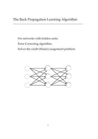
For networks with hidden units.
Error Correcting algorithm.
Solves the credit (blame) assignment problem.
1
2. What is supervised learning?
Can we teach a network to learn to associate a pattern of
inputs with corresponding outputs?
i.e. given initial set of weights, how can they be adapted
to produce the desired output? Use a training set:
y
a f? d
payment
b e?
c w p
workload
person workload pay P(happy)
a 0.1 0.9 0.95
b 0.3 0.7 0.8
c 0.07 0.2 0.2
d 0.9 0.9 0.3
e 0.7 0.5 ??
f 0.4 0.8 ??
After training, how does network generalise to patterns
unseen during learning?
2
3. Learning by Error Correction
In the perceptron there was a binary valued output Ý and
a target Ø.
x1 x2 xN
w1 w2 wN
output y
target t
y
Æ 1
Ý step ÛÜ
¼
0
Σwi xi
i
Define this error measure:
½ ´Ø Ý µ¾
¾
It counts the number of incorrect outputs.
We want to design a weight changing procedure that
minimises .
3
4. Learning by Error Correction
How do we change the weights Û¼ Û½ ÛÆ so that
error decreases?
E
Suppose error
slope slope
varies with weight -ve +ve
Û like this.
wi
If we could measure the slope
Û
then changing weights by the negative of the slope will
minimise .
slope +ve ¡Û -ve move towards minimum of
slope -ve ¡Û +ve
4
5. More Perceptron Problems
For the perceptron, can’t be differentiated with respect
to weights Û¼ Û½ ÛÆ because involves output Ý
which is not differentiable.
½ ´Ø Ý µ¾ Ý step
Æ
ÛÜ
¾ ¼
Threshold Unit:
y
´ ÈÆ Û Ü 1
½ if ¼
Ý
¼ if
ÈÆ ¼ Û Ü ¼
¼
0
Σwi xi
i
Sigmoid Unit:
y
½ 1
Ý ÈÆ ¡
½ · ÜÔ ÛÜ
0
Σwi xi
i
5
6. Gradient Descent
E
The error is now slope slope
a differentiable -ve +ve
function.
wi
Change weights using negative slope
¡Û Û
Û
+ve ¡Û -ve
move towards minimum of
Û
-ve ¡Û +ve
This approach is called Gradient Descent
6
7. Derivation of Back Propagation
x1 v1 y1
x2 v2 y2
xk vj yi
uj k wi j
xN vN yN
inputs hidden outputs
xk vj yi
È ¡
output Ý sig Û Ú
È ¡
hidden Ú sig Ù Ü
error ½È È Ø Ý ¡¾
¾
We need to find the derivatives of with respect to weights
Û and Ù .
7
8. Preliminaries
xk ujk vj wij yi
On a single pattern (drop )
½ ¡¾
¾ Ø Ý
and
½
Ý ÈÆ ¡
½ · ÜÔ Û Ú
Note that:
Ý ¡
Ú
Ý ½ Ý Û
Ý ¡
Û
Ý ½ Ý Ú
since if Ý
½
½ · ÜÔ´ ܵ
Ý
then Ý ´½ Ý µ
Ü
8
9. Between Hidden and Output Û
xk ujk vj wij yi
For weights between hidden units
and output units.
½ ¡¾
¾ Ø Ý
Ý
Û Ý Û
¡
Ý
Ý Ø
Ý
Û
Ý ´½ ݵÚ
¡
Û
Ý Ø ßÞ ´½ Ý µ Ú
Ý
call this Æ
9
10. Between Input and Hidden Ù
xk ujk vj wij yi
For weights between input units
and hidden units.
½ ¡¾
¾ Ø Ý
Ý Ú
Ù Ý Ú Ù
¡
Ý
Ý Ø
Ý
Ú
Ý ´½ ݵÛ
Ú
Ù
Ú ´½ Ú µ Ü
¡
Ù
Ý Ø Ý ´½ Ý µ Û Ú ´½ Ú µ Ü
Ù
ÆÛ Ú ´½ Ú µ Ü
10
11. Between Hidden and Output ¡Û
xk ujk vj wij yi
Modifying weights between hidden
units and output units using
gradient descent.
¡Û Û
¡
Ý
ßÞ Ø Ý ´½
ßÞ Ý µ Ú
close to ¼ ½
small for Ý
Learning
constant
“input”
error
ßÞ
Æ
11
12. Between Input and Hidden ¡Ù
xk ujk vj wij yi
Modifying weights between input
units and hidden units using
gradient descent.
¡Ù Ù
Æ Û Ú ´½ Ú µÜ
back propagation of error
The same procedure is applicable to a net with many
hidden layers.
12
13. An Example
x1 u x2
=0 2.0
21
.8 =
u 11 =2.0 u 12
u 22 =0.8
ܽ ܾ target Ø
u 10 = -1.0 u 20 = -1.0 0 0 0
v1 v2
1 1
0 1 1
1 0 1
w1 =2.0 w2 = -1.0
1 1 0
1 y
w0 = -1.0
¡
hidden Ú½ sig Ù½½Ü½ · Ù½¾Ü¾ · Ù½¼
0.9526 ¡
Ú¾ sig Ù¾½Ü½ · Ù¾¾Ü¾ · Ù¾¼
0.6457 ¡
output Ý sig Û½Ú½ · Û¾Ú¾ · Û¼
0.5645
error ½ Ø Ý ¡¾
¾
0.1593
13
15. An Example: a New Error
x1 u x2
8
=0 1.9
21
.83 =
u 11 =1.98 u 12
u 22 =0.83
ܽ ܾ target Ø
u 10 = -1.01 u 20 = -0.96 0 0 0
v1 v2
1 1
0 1 1
1 0 1
w1 =1.86 w2 = -1.08
1 1 0
1 y
w0 = -1.13
¡
hidden Ú½ sig Ù½½Ü½ · Ù½¾Ü¾ · Ù½¼
0.9509 ¡
Ú¾ sig Ù¾½Ü½ · Ù¾¾Ü¾ · Ù¾¼
0.6672 ¡
output Ý sig Û½Ú½ · Û¾Ú¾ · Û¼
0.4776
error ½ Ø Ý ¡¾
¾
0.1140
The error has reduced for this pattern.
15
16. Summary
Credit-assignment problem solved for hidden units:
Input Output
ƽ
Û½
Û¾
Æ Æ¾
Û¿
Æ ¼
´ µÈ Û Æ Æ¿
Errors
total input to unit ; 1st derivative of acti-
¼
vation function (sigmoid)
Outstanding issues:
1. Number of layers; number and type of units in
layer
2. Learning rates
3. Local or distributed representations
16