“Semi-Flexible dense polymer brushes in flow – Simulation & Theory”, Frank Römer and Dimitry A. Fedosov, A talk given at the Institute of Physical Chemistry in Cologne, June 2015

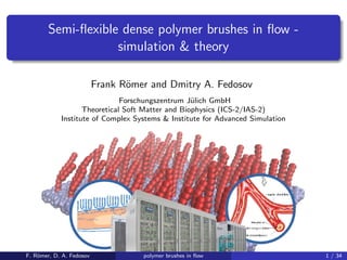
1. Semi-flexible dense polymer brushes in flow -
simulation & theory
Frank R¨omer and Dmitry A. Fedosov
Forschungszentrum J¨ulich GmbH
Theoretical Soft Matter and Biophysics (ICS-2/IAS-2)
Institute of Complex Systems & Institute for Advanced Simulation
F. R¨omer, D. A. Fedosov polymer brushes in flow 1 / 34

2. Introduction
theoretical & computational methods
from meso scale to continuum
hydrodynamic interactions
F. R¨omer, D. A. Fedosov polymer brushes in flow 2 / 34

3. Motivation
Semi-flexible polymers at high density stiff anchored onto a surface:
blood vessels lung mucus layer
inner ear
glycocalyx brush structure on the endothelial surface layer1 (EGL)
periciliary layer of the lung airway2
vestibular3 & auditory4 sensory epithelium
1
S. Weinbaum et al., Annu. Rev. Biomed. Eng. 9, 121–167 (2007).
2
B. Button et al., Science 337, 937–941 (2012).
3
K. Legendre et al., J. Cell Sci. 121, 3347–3356 (2008).
4
J. Tolomeo and M. Holley, Biophys. J. 73, 2241–2247 (1997).
F. R¨omer, D. A. Fedosov polymer brushes in flow 3 / 34

4. Motivation
Modeling blood flow in vessels with explicit EGL:
scaling problem!
→ implicit modeling or coarse graining
F. R¨omer, D. A. Fedosov polymer brushes in flow 4 / 34

5. Motivation
Can we predict the properties (e.g. height) of a dense semi-flexible
polymer brush in shear flow for a given set of parameters:
flexural rigidity EI,
grafting density σ and
shear rate ˙γ on top?
F. R¨omer, D. A. Fedosov polymer brushes in flow 5 / 34

6. Already done?
There is a lot experimental, simulation & theoretical work done on
full-flexible polymer brushes (PB), but only a few on semi-flexible PBs.
Semi-flexible polymer brushes in equilibrium:
D. V. Kuznetsov and Z. Y. Chen, J. Chem. Phys. 109, 7017–7027
(1998): scaling theory
G. G. Kim and K. Char, Bull. Korean Chem. Soc. 20, 1026–1030
(1999): continuous chain model
C.-M. Chen and Y.-A. Fwu, Phys. Rev. E 63, 011506 (2000): MC
simulation
Semi-flexible polymer brushes in flow:
Y. W. Kim et al., Macromolecules 42, 3650–3655 (2009): theory &
simulation
F. R¨omer, D. A. Fedosov polymer brushes in flow 6 / 34

7. Already done?
EI d2θ
ds2 = −3πη cos θ(s)
L
s u(s) ds
with: s2u
dy2 = 3πσ u(y)
cos θ(y)
no volume-exclusion interaction
grafting density only influence velocity
max. grafting density studied σ = 0.03
model only works for small deformations
No, it is not done!
F. R¨omer, D. A. Fedosov polymer brushes in flow 7 / 34

8. Simulations
F. R¨omer, D. A. Fedosov polymer brushes in flow 8 / 34

9. Dissipative Particle Dynamics (DPD)
simulation method
Dissipative Particle Dynamics (DPD) was introduced by Hoogerbrugge and
Koelman in 19925.
Particles in DPD represent clusters of
molecules and interact through simple
pair-wise forces: Fi = j=i (FC
ij + FR
ij + FD
ij ).
DPD system is thermally equilibrated
through a thermostat defined by forces: FR
ij
and FD
ij .
The DPD scheme consists of the calculation of the position and velocities
of interacting particles over time. The time evolution of positions and
velocities are given by: dri = vi dt and dvi = Fi dt.
5
P. Hoogerbrugge and J. Koelman, Europhys. Lett. 19, 155 (1992).
F. R¨omer, D. A. Fedosov polymer brushes in flow 9 / 34

10. Smoothed Dissipative Particle Dynamics (SDPD)
simulation method
Espa˜nol and Revenga combined in Smoothed Dissipative Particle
Dynamics (SDPD)6 best features of the Smoothed Particle
Hydrodynamics (SPH)7 and DPD methods.
SDPD allows to introduce an arbitrary equation of state:
- e.g. control compressibility.
SDPD particles has a well defined size and volume:
- consitent scaling of thermal fluctuations of the fluid,
- while dynamics of immersed objects is scale-free8
In SDPD transport coefficients (viscosity, thermal conductivity) are a
direct input.
6
P. Espa˜nol and M. Revenga, Phys. Rev. E 67, 026705 (2003).
7
R. Gingold and J. Monaghan, Mon. Not. R. Astron. Soc. 181, 375 (1977).
8
A. Vzquez-Quesada et al., J. Chem. Phys. 130, 034901 (2009).
F. R¨omer, D. A. Fedosov polymer brushes in flow 10 / 34

11. System
simulation model
The SDPD ensemble:
slit like geometry (2D PBC)
wall & fluid: SDPD particle
reflection planes at walls
Poiseuille flow in x direction:
fx,i = (dP/dx)/ρ
polymers grafted on a tetragonal lattice with alat
friction between fluid & polymer beads
We characterize the system by:
grafting density: σ = (alat/d)−2
flexibility: lp/L = EI/(kBTL)
rate: ˜˙γ = L3η ˙γ/kBT
F. R¨omer, D. A. Fedosov polymer brushes in flow 11 / 34

12. Polymer Beam
simulation model
The Polymer beam is represented by:
N = 10 + 1 tangential bonded beads of diameter d
1st two beads fixed
extensible worm-like chain model like
friction interaction with fluid
repulsive interaction between beads (WCAa)
→ volume exclusion
a
J. D. Weeks et al., J. Chem. Phys. 54, 5237–5247 (1971).
Discretized elastic potential9 for isotropic elastic cylinder of diameter d:
U ({rk}) = N−1
i=0
kb
2d [ri,i+1 − d]2
+ EI
d [1 − cos ∆θ]
with: EI/kb = d2/16
9
X. Schlagberger and R. R. Netz, Europhys. Lett. 70, 129 (2005).
F. R¨omer, D. A. Fedosov polymer brushes in flow 12 / 34

13. Results
We have simulated systems with:
grafting densities σ from 0.01 to 1,
and beam elasticities lp/L of 10 and 100
at shear rates ˜˙γ between 101 and 106.
The Reynolds number, referring to the maximum velocity the polymer
brush is exposed at the tip and beam elasticity, varies between
Re = ρud
η = impulsconvection
diffusion = 10−6 − 10−1 → Stokes regime10.
Height of brush is calculated from the first moment of the polymer
monomer density profile11:
h = 2
yρ(y)dy
ρ(y)dy
10
E. Guyon et al., Physical hydrodynamics, (Oxford University Press, 2001).
11
M. Deng et al., J. Fluid Mech. 711, 192–211 (2012).
F. R¨omer, D. A. Fedosov polymer brushes in flow 13 / 34

14. Results
comparison of methods
Comparison with LB and BD simulations from Y. W. Kim et al.,
Macromolecules 42, 3650–3655 (2009):
F. R¨omer, D. A. Fedosov polymer brushes in flow 14 / 34

15. Results
from SDPD simulations
Polymer brush height as a function of shear rate on top of the brush:
F. R¨omer, D. A. Fedosov polymer brushes in flow 15 / 34

16. Theory
F. R¨omer, D. A. Fedosov polymer brushes in flow 16 / 34

17. Theoretical Model
The polymer beam is treated as a cantilever.
Uniform behavior
Quasi 2D: no perturbation in z
Internal coordinates along
contour line: s, θ(s)
Euler-Bernoulli beam theory:
EI dr(s)
ds × d3r(s)
ds3 = F(s) × dr(s)
ds
EI d2θ(s)
ds2 = Fy (s) sin θ(s) − Fx (s) cos θ(s)
Hydrodynamic drag force: Fd(s)
Volume exclusion force: Fv(s)
Boundary conditions:
θ(s)|s=0 = 0 at the grafting surface, and dθ/ds|s=L = 0 at the free end.
F. R¨omer, D. A. Fedosov polymer brushes in flow 17 / 34

18. Shear force on the beam
theoretical model
The effective shear force acting on the beam at
position s:
Fd(s) =
L
s fd(s )ds,
with the local force density due to hydrodynamic
interaction for the x-component
f d
x (s) = f d
⊥(s) cos θ(s) + f d(s) sin θ(s),
and the y-component
f d
y (s) = f d
⊥(s) sin θ(s) − f d(s) cos θ(s)
F. R¨omer, D. A. Fedosov polymer brushes in flow 18 / 34

19. Shear force on the beam
theoretical model
Shear force components:
f d
⊥(s) = ζ⊥(s)ηux (s) cos θ(s) and f d(s) = ζ (s)ηux (s) sin θ(s)
Friction coefficient from slender body theorya,
piecewise approximated as a cylinderb:
ζ⊥ = 8π
ln(L/d)−1
2
+ln(2)
,
ζ = 4π
ln(L/d)−3
2
+ln(2)
.
a
R. G. Cox, J. Fluid Mech. 44, 791–810 (1970).
b
C. H. Wiggins et al., Biophys. J. 74, 1043–1060 (1998).
Local velocity ux (s) depend on the hydrodynamic
penetrationc.
c
S. T. Milner, Macromolecules 24, 3704–3705 (1991).
F. R¨omer, D. A. Fedosov polymer brushes in flow 19 / 34

20. Velocity profile
theoretical model
Local velocity u(s) depend on the hydrodynamic penetration into the
brush12:
Like Kim et al.13 we introduce an equation similar to the Brinkman
equation14 for flow in porous media but depending on local density:
d2u
dy2 = ζσ u(y)
cos θ(y) → d2ux (s)
ds2 = ζ(s)ux (s) σ
d2 cos θ(s) − dux (s)
ds
dθ(s)
ds tan θ(s),
with boundary conditions: u(y)|y=0 = u(s)|s=0 = 0, and du/dy|y=L = ˙γL
resp. du/ds|s=L = ˙γL sin θ(L).
12
S. T. Milner, Macromolecules 24, 3704–3705 (1991).
13
Y. W. Kim et al., Macromolecules 42, 3650–3655 (2009).
14
H. C. Brinkman, Appl. Sci. Res. A1 A1, 27 (1947).
F. R¨omer, D. A. Fedosov polymer brushes in flow 20 / 34

21. Volume exclusion
theoretical model
Discretise the beam: N = L/d spheres
Positions are given as a function of s:
the f
x(s) =
s
0 sin θ(s )ds ∧ y(s) =
s
0 cos θ(s )ds
Assume a repulsive interaction:
gij =
rij d : g
kB T
d [(d/rij )α
− 1]
rij
rij
rij > d : 0
with g 50 and α ≥ 3.
Force density fv
n on a sphere n ∈ [0...N − 1] in
a discretized beam:
fv
n = j
gnj
d
Fv(s) = fv
s/d (d s/d − s/d) + N−1
n= s/d fv
n d
F. R¨omer, D. A. Fedosov polymer brushes in flow 21 / 34

22. Theoretical Solution
Brinkman-like equation
d2ux (s)
ds2 = ζ(s)ux (s) σ
d2 cos θ(s) − dux (s)
ds
dθ(s)
ds tan θ(s)
Beam equation
EI d2θ(s)
ds2 = Fy (s) sin θ(s) − Fx (s) cos θ(s)
Solver scheme:
0 guess a configuration: θ0(s) for s ∈ [0, L]
1 calculate volume exclusion force → Fv(s)
2 solve Brinkman-like equation → u(s) ⇒ Fd(s)
3 Beam equation & DuFort-Frankel scheme15 → θn(s)
4 if
L
0 |θn − θn−1| ds > tol : goto 1 else : found final configuration ;)
15
E. C. Du Fort and S. P. Frankel, Math. Comp. 7, 135–152 (1953).
F. R¨omer, D. A. Fedosov polymer brushes in flow 22 / 34

23. Results
SDPS vs theory
Comparison between SDPD simulation and our theoretical model:
brush height
Figure : Relative brush height vs shear rate normalized by polymer elasticity
F. R¨omer, D. A. Fedosov polymer brushes in flow 23 / 34

24. Results
SDPS vs theory
Comparison between SDPD simulation and our theoretical model:
brush height
overestimation of volume-exclusion term Fv ← neglected perturbation in z
F. R¨omer, D. A. Fedosov polymer brushes in flow 24 / 34

25. Results
error analysis
Figure : Relative deviation of brush height vs shear rate.
N 106
RMS 14.6 %
AAD 9.5 %
Bias 8.3 %
F. R¨omer, D. A. Fedosov polymer brushes in flow 25 / 34

26. Results
theoretical model
Prediction of the response to shear flow of dense polymer brushes.
EGL, σ ≈ 1
F. R¨omer, D. A. Fedosov polymer brushes in flow 26 / 34

27. Results
SDPS vs theory
Comparison between SDPD simulation and our theoretical model:
velocity profile
Figure : normalized velocity profiles, ∂P/∂x = const.
F. R¨omer, D. A. Fedosov polymer brushes in flow 27 / 34

28. Results
theoretical model
Prediction of flow rates in channels or tubes.
micro-vascular flow
F. R¨omer, D. A. Fedosov polymer brushes in flow 28 / 34

29. Results
SDPS vs theory
Comparison between SDPD simulation and our theoretical model:
Relative apparent viscosity
Figure : Relative apparent viscosity vs shear rate scaled by elasticity.
F. R¨omer, D. A. Fedosov polymer brushes in flow 29 / 34

30. Results
theoretical model
Prediction of app. viscosity as input for continuous methods.
microfluidic devices
F. R¨omer, D. A. Fedosov polymer brushes in flow 30 / 34

31. Conclusion
Simulations of polymer brushes with
densities varying between 0.01 (no interaction between polymers)
and 1 (maximum density of SC packing),
with elasticities in range of 2 orders of magnitude and
under top shear loads in range of 6 orders of magnitude.
Simulations h(σ, EI, ˙γ) in good agreement with previous studies.
We propose the first theoretical model describing dense semi-flexible
polymer brushes in a wide parameter range:
Good agreement with simulations: (∆h)max ≈ d.
Model reproduces all features shown in simulation.
Systematic overestimation of height due to reduced dimensionality.
Now we can predict the interaction of a dense
semi-flexible polymer brush with shear flow!
F. R¨omer and D. A. Fedosov, Europhysics Letters 109, 68001 (2015)
F. R¨omer, D. A. Fedosov polymer brushes in flow 31 / 34

32. Outlook
Direct mechanical stress or deformation of the brush.
→ simulation of brush compression:
preliminary results in good
agreement with theoretical model
⇒ add viscoelasticity to vessel walls:
model mechanical transduction of
forces due to e.g. EGL–RBC
interactions
F. R¨omer, D. A. Fedosov polymer brushes in flow 32 / 34

33. Acknowledgements
D. A. Fedosov
co-author
J¨ulich Supercomputing Centre (JSC)
F. R¨omer, D. A. Fedosov polymer brushes in flow 33 / 34

34. F. R¨omer, D. A. Fedosov polymer brushes in flow 34 / 34