maxbox starter60 machine learning
•
0 likes•98 views

This document provides an overview of machine learning concepts and code examples in Python. It discusses the typical 5 steps of machine learning projects: collaboration, data collection, clustering, classification, and conclusion. Code snippets demonstrate each step, including collecting data with Scrapy, clustering with k-means, classification with support vector machines, and evaluating results with a confusion matrix. Dimensionality reduction techniques like principal component analysis are also covered.
![maXbox4 4.6.2.10 26/02/2018 23:22:21
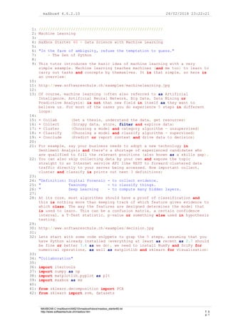
43: from sklearn.model_selection import train_test_split
44: from sklearn.metrics import confusion_matrix
45: from scipy import special, optimize
46:
47: Then we go like this 5 steps:
48:
49: • Collab (Python and maXbox as a tool)
50: • Collect (from scrapy.crawler import CrawlerProcess)
51: • Cluster (clustering with K-Means - unsupervised)
52: • Classify (classify with Support Vector Machines - supervised)
53: • Conclude (test with a Confusion Matrix)
54:
55:
56: "Collecting"
57:
58: class BlogSpider(scrapy.Spider):
59: name = 'blogspider'
60: start_urls = ['https://blog.scrapinghub.com']
61:
62: def parse(self, response):
63: for title in response.css('h2.entry-title'):
64: yield {'title': title.css('a ::text').extract_first()}
65:
66: for next_page in response.css('div.prev-post > a'):
67: yield response.follow(next_page, self.parse)
68: print(next_page)
69:
70: We are going to create a class called LinkParser that inherits some
methods from HTMLParser which is why it is passed into the definition.
This snippet can be used to run scrapy spiders independent of scrapyd or
the scrapy command line tool and use it from a script.
71:
72:
73: "Clustering"
74:
75: def createClusteredData(N, k):
76: pointsPerCluster = float(N)/k
77: X = []
78: y = []
79: for i in range (k):
80: incomeCentroid = np.random.uniform(20000.0, 200000.0)
81: ageCentroid = np.random.uniform(20.0, 70.0)
82: for j in range(int(pointsPerCluster)):
83: X.append([np.random.normal(incomeCentroid, 10000.0),
84: np.random.normal(ageCentroid, 2.0)])
85: y.append(i)
86: X = np.array(X)
87: y = np.array(y)
88: print('Cluster uniform, with normalization')
89: print(y)
90: return X, y
91:
92: The 2 arrays you can see is X as the feature array and y as the predict
array (array object as a list)! We create a fake income / age clustered
data that we use for our K-Means clustering example above for the
simplicity.
93:
94:
95: "Classification"
96:
97: Now we will use linear SVC to partition our graph into clusters and split
the data into a training set and a test set for further predictions.
MAXBOX8 C:maXboxmX46210maxbox4docsmaxbox_starter60.txt
http://www.softwareschule.ch/maxbox.htm T: 5
p: 2](data:image/gif;base64,R0lGODlhAQABAIAAAAAAAP///yH5BAEAAAAALAAAAAABAAEAAAIBRAA7)
Recommended
Recommended
More Related Content
What's hot
What's hot (20)
Similar to maxbox starter60 machine learning
Similar to maxbox starter60 machine learning (20)
More from Max Kleiner
More from Max Kleiner (20)
Recently uploaded
Recently uploaded (20)
maxbox starter60 machine learning
- 1. maXbox4 4.6.2.10 26/02/2018 23:22:21 1: ////////////////////////////////////////////////////// 2: Machine Learning 3: ______________________________________________________ 4: maXbox Starter 60 - Data Science with Machine Learning 5: 6: "In the face of ambiguity, refuse the temptation to guess." 7: - The Zen of Python 8: 9: This tutor introduces the basic idea of machine learning with a very simple example. Machine learning teaches machines (and me too) to learn to carry out tasks and concepts by themselves. It is that simple, so here is an overview: 10: 11: http://www.softwareschule.ch/examples/machinelearning.jpg 12: 13: Of course, machine learning (often also referred to as Artificial Inteligence, Artificial Neural Network, Big Data, Data Mining or Predictive Analysis) is not that new field in itself as they want to believe us. For most of the cases you do experience 5 steps in different loops: 14: 15: • Collab (Set a thesis, understand the data, get resources) 16: • Collect (Scrapy data, store, filter and explore data) 17: • Cluster (Choosing a model and category algorithm - unsupervised) 18: • Classify (Choosing a model and classify algorithm - supervised) 19: • Conclude (Predict or report context and drive data to decision) 20: 21: For example, say your business needs to adopt a new technology in Sentiment Analysis and there’s a shortage of experienced candidates who are qualified to fill the relevant positions (also known as a skills gap). 22: You can also skip collecting data by your own and expose the topic straight to an Internet service API like REST to forward clustered data traffic directly to your server being accessed. How important collect, cluster and classify is points out next 3 definitions; 23: 24: "Definition: Digital Forensic - to collect evidence. 25: " Taxonomy - to classify things. 26: " Deep Learning - to compute many hidden layers. 27: 28: At its core, most algorithms should have a proof of classification and this is nothing more than keeping track of which feature gives evidence to which class. The way the features are designed determines the model that is used to learn. This can be a confusion matrix, a certain confidence interval, a T-Test statistic, p-value or something else used in hypothesis testing. 29: 30: http://www.softwareschule.ch/examples/decision.jpg 31: 32: Lets start with some code snippets to grap the 5 steps, assuming that you have Python already installed (everything at least as recent as 2.7 should be fine or better 3.6 as we do), we need to install NumPy and SciPy for numerical operations, as well as matplotlib and sklearn for visualization: 33: 34: "Collaboration" 35: 36: import itertools 37: import numpy as np 38: import matplotlib.pyplot as plt 39: import maxbox as mx 40: 41: from sklearn.decomposition import PCA 42: from sklearn import svm, datasets MAXBOX8 C:maXboxmX46210maxbox4docsmaxbox_starter60.txt http://www.softwareschule.ch/maxbox.htm T: 5 p: 1
- 2. maXbox4 4.6.2.10 26/02/2018 23:22:21 43: from sklearn.model_selection import train_test_split 44: from sklearn.metrics import confusion_matrix 45: from scipy import special, optimize 46: 47: Then we go like this 5 steps: 48: 49: • Collab (Python and maXbox as a tool) 50: • Collect (from scrapy.crawler import CrawlerProcess) 51: • Cluster (clustering with K-Means - unsupervised) 52: • Classify (classify with Support Vector Machines - supervised) 53: • Conclude (test with a Confusion Matrix) 54: 55: 56: "Collecting" 57: 58: class BlogSpider(scrapy.Spider): 59: name = 'blogspider' 60: start_urls = ['https://blog.scrapinghub.com'] 61: 62: def parse(self, response): 63: for title in response.css('h2.entry-title'): 64: yield {'title': title.css('a ::text').extract_first()} 65: 66: for next_page in response.css('div.prev-post > a'): 67: yield response.follow(next_page, self.parse) 68: print(next_page) 69: 70: We are going to create a class called LinkParser that inherits some methods from HTMLParser which is why it is passed into the definition. This snippet can be used to run scrapy spiders independent of scrapyd or the scrapy command line tool and use it from a script. 71: 72: 73: "Clustering" 74: 75: def createClusteredData(N, k): 76: pointsPerCluster = float(N)/k 77: X = [] 78: y = [] 79: for i in range (k): 80: incomeCentroid = np.random.uniform(20000.0, 200000.0) 81: ageCentroid = np.random.uniform(20.0, 70.0) 82: for j in range(int(pointsPerCluster)): 83: X.append([np.random.normal(incomeCentroid, 10000.0), 84: np.random.normal(ageCentroid, 2.0)]) 85: y.append(i) 86: X = np.array(X) 87: y = np.array(y) 88: print('Cluster uniform, with normalization') 89: print(y) 90: return X, y 91: 92: The 2 arrays you can see is X as the feature array and y as the predict array (array object as a list)! We create a fake income / age clustered data that we use for our K-Means clustering example above for the simplicity. 93: 94: 95: "Classification" 96: 97: Now we will use linear SVC to partition our graph into clusters and split the data into a training set and a test set for further predictions. MAXBOX8 C:maXboxmX46210maxbox4docsmaxbox_starter60.txt http://www.softwareschule.ch/maxbox.htm T: 5 p: 2
- 3. maXbox4 4.6.2.10 26/02/2018 23:22:21 98: 99: X_train, X_test, y_train, y_test = train_test_split(X, y, random_state=0) 100: 101: # Run classifier, using a model that is too regularized (C too low) to see 102: # the impact on the results 103: 104: classifier = svm.SVC(kernel='linear', C=0.01) 105: y_pred = classifier.fit(X_train, y_train).predict(X_test) 106: 107: By setting up a dense mesh of points in the grid and classifying all of them, we can render the regions of each cluster as distinct colors: 108: 109: def plotPredictions(clf): 110: xx, yy = np.meshgrid(np.arange(0, 250000, 10), 111: np.arange(10, 70, 0.5)) 112: Z = clf.predict(np.c_[xx.ravel(), yy.ravel()]) 113: 114: plt.figure(figsize=(8, 6)) 115: Z = Z.reshape(xx.shape) 116: plt.contourf(xx, yy, Z, cmap=plt.cm.Paired, alpha=0.8) 117: plt.scatter(X[:,0], X[:,1], c=y.astype(np.float)) 118: plt.show() 119: 120: It returns coordinate matrices from coordinate vectors. Make N-D coordinate arrays for vectorized evaluations of N-D scalar/vector fields over N-D grids, given one-dimensional coordinate arrays x1, x2,..., xn. 121: Or just use predict for a given point: 122: 123: print(svc.predict([[100000, 60]])) 124: print(svc.predict([[50000, 30]])) 125: 126: 127: "Conclusion" 128: 129: The last step as an example of confusion matrix usage to evaluate the quality of the output on the data set. The diagonal elements represent the number of points for which the predicted label is equal to the true label, while off-diagonal elements are those that are mislabeled by the classifier. The higher the diagonal values of the confusion matrix the better, indicating many correct predictions. 130: 131: def plot_confusion_matrix(cm, classes, 132: normalize=False, 133: title='Confusion matrix', 134: cmap=plt.cm.Blues): 135: """ 136: This function prints and plots the confusion matrix. 137: Normalization can be applied by setting `normalize=True`. 138: """ 139: if normalize: 140: cm = cm.astype('float') / cm.sum(axis=1)[:, np.newaxis] 141: print("Normalized confusion matrix") 142: else: 143: print('Confusion matrix, without normalization') 144: 145: print(cm) 146: 147: 148: "Comprehension" 149: 150: A last point is dimensionality reduction as the plot on http://www.softwareschule.ch/examples/machinelearning.jpg shows, its more a preparation but could also necessary to data reduction or to find a thesis. MAXBOX8 C:maXboxmX46210maxbox4docsmaxbox_starter60.txt http://www.softwareschule.ch/maxbox.htm T: 5 p: 3
- 4. maXbox4 4.6.2.10 26/02/2018 23:22:21 151: 152: Principal component analysis (PCA) is often the first thing to try out if you want to cut down number of features and do not know what feature extraction method to use. 153: PCA is limited as its a linear method, but chances are that it already goes far enough for your model to learn well enough. 154: Add to this the strong mathematical properties it offers and the speed at which it finds the transformed feature data space and is later able to transform between original and transformed features; we can almost guarantee that it also will become one of your frequently used machine learning tools. 155: 156: This tutor will go straight to an overview to PCA. 157: 158: The script 811_mXpcatest_dmath_datascience.pas (pcatest.pas) (located in the democonsolecurfit subdirectory) performs a principal component analysis on a set of 4 variables. Summarizing it, given the original feature space, PCA finds a linear projection of itself in a lower dimensional space that has the following two properties: 159: 160: • The conserved variance is maximized. 161: • The final reconstruction error (when trying to go back from transformed 162: features to the original ones) is minimized. 163: 164: As PCA simply transforms the input data, it can be applied both to classification and regression problems. In this section, we will use a classification task to discuss the method. 165: 166: The script can be found at: 167: http://www.softwareschule.ch/examples/811_mXpcatest_dmath_datascience.pas 168: ..examples811_mXpcatest_dmath_datascience.pas 169: 170: It may be seen that: 171: 172: • High correlations exist between the original variables, which are 173: therefore not independent 174: 175: • According to the eigenvalues, the last two principal factors may be 176: neglected since they represent less than 11 % of the total variance. So, 177: the original variables depend mainly on the first two factors 178: 179: • The first principal factor is negatively correlated with the second and 180: fourth variables, and positively correlated with the third variable 181: 182: • The second principal factor is positively correlated with the first 183: variable 184: 185: • The table of principal factors show that the highest scores are usually 186: associated with the first two principal factors, in agreement with the 187: previous results 188: 189: Const 190: N = 11; { Number of observations } 191: Nvar = 4; { Number of variables } 192: 193: Of course, its not always this and that simple. Often, we dont know what number of dimensions is advisable in upfront. In such a case, we leave n_components or Nvar parameter unspecified when initializing PCA to let it calculate the full transformation. After fitting the data, explained_variance_ratio_ contains an array of ratios in decreasing order: The first value is the ratio of the basis vector describing the direction of the highest variance, the second value is the ratio of the direction of the second highest variance, and so on. MAXBOX8 C:maXboxmX46210maxbox4docsmaxbox_starter60.txt http://www.softwareschule.ch/maxbox.htm T: 5 p: 4
- 5. maXbox4 4.6.2.10 26/02/2018 23:22:21 194: 195: Being a linear method, PCA has, of course, its limitations when we are faced with strange data that has non-linear relationships. We wont go into much more details here, but its sufficient to say that there are extensions of PCA. 196: 197: 198: Ref: 199: Building Machine Learning Systems with Python 200: Second Edition March 2015 201: 202: DMath Math library for Delphi, FreePascal and Lazarus May 14, 2011 203: 204: http://www.softwareschule.ch/box.htm 205: http://fann.sourceforge.net 206: http://neuralnetworksanddeeplearning.com/chap1.html 207: 208: Doc: 209: Neural Networks Made Simple: Steffen Nissen 210: http://fann.sourceforge.net/fann_en.pdf 211: http://www.softwareschule.ch/examples/datascience.txt 212: https://maxbox4.wordpress.com 213: https://www.tensorflow.org/ 214: 215: 216: https://sourceforge.net/projects/maxbox/files/Examples/13_General 217: /811_mXpcatest_dmath_datascience.pas/download 218: https://sourceforge.net/projects/maxbox/files/Examples/13_General 219: /809_FANN_XorSample_traindata.pas/download 220: https://stackoverflow.com/questions/13437402/how-to-run-scrapy-from-within- a-python-script 221: 222: 223: Plots displaying the explained variance over the number of components is called a Scree plot. A nice example of combining a Screeplot with a grid search to find the best setting for the classification problem can be found at 224: 225: http://scikit- learn.sourceforge.net/stable/auto_examples/plot_digits_pipe.html. 226: 227: Although, PCA tries to use optimization for retained variance, multidimensional scaling (MDS) tries to retain the relative distances as much as possible when reducing the dimensions. This is useful when we have a high-dimensional dataset and want to get a visual impression. 228: 229: Machine learning is the science of getting computers to act without being explicitly programmed. In the past decade, machine learning has given us self-driving cars, practical speech recognition, effective web search, and a vastly improved understanding of the human genome. Machine learning is so pervasive today that you probably use it dozens of times a day without knowing it. 230: 231: >>> Building Machine Learning Systems with Python 232: >>> Second Edition MAXBOX8 C:maXboxmX46210maxbox4docsmaxbox_starter60.txt http://www.softwareschule.ch/maxbox.htm T: 5 p: 5