Feedback and Control Systems Matlab Handouts #2

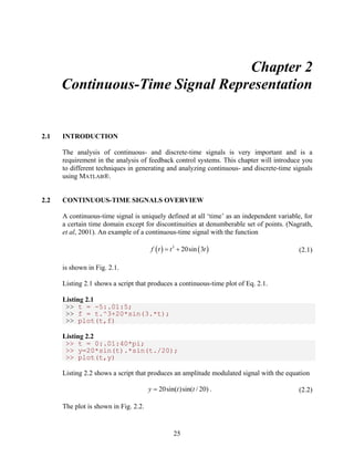
1. 25
Chapter 2
Continuous-Time Signal Representation
2.1 INTRODUCTION
The analysis of continuous- and discrete-time signals is very important and is a
requirement in the analysis of feedback control systems. This chapter will introduce you
to different techniques in generating and analyzing continuous- and discrete-time signals
using MATLAB®.
2.2 CONTINUOUS-TIME SIGNALS OVERVIEW
A continuous-time signal is uniquely defined at all ‘time’ as an independent variable, for
a certain time domain except for discontinuities at denumberable set of points. (Nagrath,
et al, 2001). An example of a continuous-time signal with the function
f (t ) = t3 + 20sin (3t ) (2.1)
is shown in Fig. 2.1.
Listing 2.1 shows a script that produces a continuous-time plot of Eq. 2.1.
Listing 2.1
>> t = -5:.01:5;
>> f = t.^3+20*sin(3.*t);
>> plot(t,f)
Listing 2.2
>> t = 0:.01:40*pi;
>> y=20*sin(t).*sin(t./20);
>> plot(t,y)
Listing 2.2 shows a script that produces an amplitude modulated signal with the equation
y = 20sin(t)sin(t / 20) . (2.2)
The plot is shown in Fig. 2.2.

2. Fig. 2.1 An example of a continuous-time signal.
Fig. 2.2 An example of an amplitude-modulated signal.
26

3. A t
 >
=  < 
27
2.3 SOME IDEAL SIGNALS
Step Function
Fig. 2.3 A plot of the step function with amplitude of 10.0.
A step function represents a sudden change as indicated in Fig. 2.3. It is mathematically
defined as
( ) , 0
s 0, 0
f t
t
(2.3)
where, A is the amplitude of the function. If the amplitude A is 1.0, then the function is
called a unit step function, which is sometimes denoted as u(t). A step function with
amplitude of 10.0 can be plotted using the listing below.
Listing 2.3
>> t = -5:0.01:10;
>> y = [zeros(1,length(-5:0.01:0-0.01))…
10*ones(1,length(0:0.01:10))];
>> plot(t,y,’+’)
Since the entire function will be a vector of values (which is actually 1501 values), it is
better divide the vector into two: a sub-vector of ‘0’s as the first element, and a sub-vector
of ‘1’s as the second element. The idea is to first generate a sub-vector of ‘1’
which is possibly done with ones(1,length(0:0.01:10)). This sub-vector will

4. be the second element of the step function vector to be generated. This will produce 1001
copies of ‘1’s in the vector. The next step is to generate a sub-vector of ‘0’s which is
possibly done with zeros(1,length(-5:0.01:0-0.01)). This sub-vector will
be the first element of the step function vector. Finally, a multiplicative factor of 10.0 is
multiplied in the sub-vector of ‘1’s.
Listing 2.3 is a straightforward way of generating a step function. Another method is by
first defining the two sub-vectors in a two variables. The two variables are then used as
the two entries in the step function vector.
Listing 2.4
>> t = -5:0.01:10;
>> y1 = zeros(1,length(-5:0.01:0-0.01));
>> y2 = 10*ones(1,length(0:0.01:10));
>> y = [y1 y2];
>> plot(t,y,’+’)
28
Ramp Function
Fig. 2.4 A plot of the ramp function with a multiplicative factor of 2.0.
A ramp function is a function that increases in amplitude as time increases from zero to
infinity. It is mathematically defined as

5. At t
( ) , 0
s 0, 0
 >
=  < 
=  +φ 
29
f t
t
(2.4)
where, A is a multiplicative factor that dictates the steepness of the ramp. If A is 1.0, the
ramp function is called a unit ramp function. An example of a ramp function with a
multiplicative factor of 2.0 is shown in Fig. 2.4. The MATLAB® script is shown in Listing
2.5.
Listing 2.5
>> t1=-5:0.01:0-0.01;
>> t2=0:0.01:10;
>> t=[t1 t2];
>> y1 = zeros(1,length(t1));
>> y2 = 2*ones(1,length(t2)).*t2;
>> y=[y1 y2];
>> plot(t,y,’+’)
Sine Wave (Sinusoidal) Function
A sinusoidal function is expressed as
π
x (t ) Asin 2 t
T
 
(2.5)
where, A is the amplitude of the sinusoid, T is the fundamental period of the wave in
seconds, and φ is the phase angle in radians. Since the fundamental period is equal to the
reciprocal of the fundamental frequency, the sinusoid can be expressed as
x (t ) = Asin (2π ft +φ ) = Asin (ωt +φ ) (2.6)
where, f is the fundamental frequency, and ω is the frequency in rad/s.
An example of a sinusoid with the function
x (t ) = 5sin (t )
is shown in Fig. 2.5. The sinusoidal signal has a fundamental period of 2π Hertz. The
Matlab® script is shown in Listing 2.6.
Listing 2.6
>> t=0:2*pi/100:4*pi;
>> y=5*sin(t);
>> plot(t,y)

6. Fig. 2.5 An example of a sinusoid.
30
2.4 EXERCISES
1. Generate a step function with an amplitude of 5.0. Plot the signal at the range of
−10 ≤ t ≤ 20 seconds with a resolution of 0.01 secs.
2. Make a delay shift to the step function generated in No. 1 by 2 secs. Plot the signal at
the range and resolution given in No. 1.
3. Generate a pulse train with a period of 5 secs. and a duty cycle of 50%. Plot the pulse
train at the range of 0 ≤ t ≤ 20 with a resolution of 0.01 secs.
4. Plot the function x (t ) = 2cos (100π t ) +1 . The plot must show only the first five
periods of the sinusoid.
5. Generate a sequence of impulses with amplitude of 1.0 at the range of 0 ≤ t ≤ 5
seconds with a resolution of 0.01 secs. The interval between pulses in 1 sec.