Making Maps for Campus Collaborations

This presentation, given at the QQML 2014 conference in Istanbul, describes a collaborative Google mapping project between the University of Arkansas Libraries and the University's Office of International Students and Scholars (OISS). Using data on the current number of international students by country of origin provided by the OISS, we created a graduated color world map visualizing this information with Google Fusion Tables. The resulting map has been embedded in a web page on the OISS website and displayed on a large touch-screen panel in the student union during International Education Week. This presentation gives step-by-step instructions for easily creating such maps - a service which libraries might offer as a basis for campus outreach and collaborative projects.

Recomendados
Mais conteúdo relacionado
Semelhante a Making Maps for Campus Collaborations
Semelhante a Making Maps for Campus Collaborations (20)
Mais de Kate Dougherty
Mais de Kate Dougherty (8)
Último
Último (20)
Making Maps for Campus Collaborations
- 1. Making Maps for Campus Collaborations 2014 International QQML Conference, Istanbul Kate Dougherty, University of Arkansas
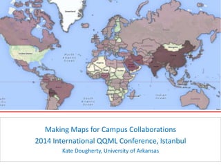
- 2. International Students Map • Map of University of Arkansas international students by country • Library’s Diversity Committee outreach to the Office of International Students & Scholars (OISS) • Embedded in OISS website; large panel in Union • Semester basis – 3 maps to date
- 4. Google Fusion Tables • Extension to Google Drive; Beta • Upload a table of your own data – Visualize as a chart, graph or map – Or, merge or “fuse” your data with a public dataset on Google Drive
- 5. Prepared Excel Spreadsheet • Entered zeroes in blank spaces • Made sure numbers are formatted as numbers • Added a column for the 3-letter ISO country codes
- 6. Create Table: Preview Columns
- 7. Create Table: Enter Metadata
- 8. Create Table: Preview • Auto-detected location/geographic info is highlighted • A new tab for a map view is automatically added
- 10. Default Map View • Points in center of each country • We wanted: countries colored in, with intensity reflecting no. of students • Additional step: merge our table with a public dataset having country outlines
- 11. Find a Public Table to Merge With
- 12. View Suggested Tables • By default, Google suggests public tables matching on the leftmost column. • ISO code in our case
- 13. Choosing a Public Table • Needed 100% matching rows across both tables (all countries in orig. spreadsheet) • Previewed with "view table" link • Looked for geographic keywords: “KML”, “geometry”, lat/long etc.
- 14. Preview Public Table: No Map Info • This table just has country names and codes • No lat/long or geographic keywords • Moving on…
- 15. Searching for Public Tables • Keyword search: – “borders" – "boundaries" – "international” • Looked for geographic keywords in results • Preview table
- 17. Preview: Zoomed Far Out
- 18. Preview: Zoomed in to Larger Scale
- 19. Select Table to Merge With
- 20. Merge Tables • Merged tables based on 3- letter country code field
- 21. Choose Columns to Merge • Deselected unwanted columns from the public table
- 23. Visualize Merged Table as a Map
- 24. Style Features
- 25. Color by Student Total
- 26. Gradient – Option 1
- 27. Buckets – Option 2: More Control
- 28. Countries with No Students Transparent
- 29. Style the Info Window
- 30. Remove Columns from Display
- 31. HTML Editor for Custom Styles
- 32. New Info Window-Map Finished!
- 33. Sharing the Map
- 34. Set Permissions: Public Status
- 35. Publish Map
- 36. Other Potential Collaborative Projects • Campus sustainability projects and green buildings • Study abroad • Language programs • Rare book exhibits • Teaching faculty’s field work locations, intl. fellowships or conference presentations • Offer to embed interactive maps in course/topic LibGuides – Greek & German sites for Intro to Philosophy – History – Archaeology – Important geologic sites
- 37. THANK YOU! Kate Dougherty Geosciences and Maps Librarian University of Arkansas kmdoughe@uark.edu @kate_dougherty
Notas do Editor
- Google Drive is Google’s cloud-based document storage, sharing and re-use platform.
- So first we prepared our spreadsheet, which involved…
- Previewed and confirmed our column headers.
- Google prompts for a table name, export permissions, a data attribution and table description. The attribution fields are limited to one source, and we had three, so we added that information to the description.
- So on the right is what our imported table looks like. Google auto-detects and highlights location information. So Google knows the countries are locations, and has automatically added a map view. As I mentioned before, FT allows you to visualize your data in different ways, and you can do this by adding tabs for different views.
- Borders can be represented in a table by lat/long coordinates for each point, or vertex.
- So the next step was to find a publicly available table submitted by someone else that had that info, and that can be done under the File menu.
- …that’s the unique identifier for each country, which would be the best way to match…
- “Geometry” may not sound like a geographic term, but features on a map are based on geometry/shapes: points for cities, lines for roads, and polygons for borders.
- So this is one of the tables we previewed, and you can see it just has…
- So we didn’t find any suggested tables that met our criteria, so we did a keyword search, using terms like…
- So we previewed the table and saw that there’s a geometry column with KML info, and the one next to it is the “geometry vertex count” or number of vertices in each boundary. There’s also lat/long. It looked great, so we took a look at the map tab…
- Automatically zooms really far out so it looks weird at first – need to zoom in to a larger scale before you can see the boundaries.
- So they all looked uniform at this point, but after merging our table with this one we would be able to shade each country by total # of students.
- So we went ahead and chose this table…
- And matched them up based on the 3-letter ISO code field.
- Click on the link to view your new, merged table that will appear when Google has completed the merge.
- So this was our new, joined table with the headers for the new columns highlighted…we then looked at the map view…
- This screen shot is zoomed out a bit far, but it still looks like the first version – just points. We then had to change the feature style to polygon.
- …but they were still uniformly colored. There are a few options for changing this – the easiest is to use a gradient.
- So that’s what we tried first, and this is what it looks like, but it doesn’t let you exclude zero values, and we wanted countries with zero students to appear transparent. So we used buckets instead, which give you a lot more control…
- So we used a custom number of “buckets” for our values, and specified the column we wanted those values to come from. The shading defaults to a value range of 1-100, and we had to click the link for “use this rage” to specify that we wanted to use the actual range of data in that column, rather than a 1-100 scale.
- And we were able to create a “bucket” just for zero values and make it transparent.
- So we styled our features, and the next step was to style the information window.
- You can remove columns from the display just by unchecking them here.
- And if you’re so inclined, you can also go to the “Custom” tab to style the window with HTML.
- So that’s it – this is how the finished map looks.
- So at this point we shared the map. There are actually 2 steps to doing this…first, we used the share button…
- …and changed its status to “public on the web”.
- Then we had to “publish” it to get embed code and a link.
- So some other potential projects that could be done with this include…