An applied two dimensional b-spline model for interpolation of data

International Journal of Advanced Research in Engineering and Technology (IJARET), ISSN 0976 –
INTERNATIONAL JOURNAL OF ADVANCED RESEARCH IN
6480(Print), ISSN 0976 – 6499(Online) Volume 3, Number 2, July-December (2012), © IAEME
ENGINEERING AND TECHNOLOGY (IJARET)
ISSN 0976 - 6480 (Print)
ISSN 0976 - 6499 (Online)
IJARET
Volume 3, Issue 2, July-December (2012), pp. 322-336
© IAEME: www.iaeme.com/ijaret.asp ©IAEME
Journal Impact Factor (2012): 2.7078 (Calculated by GISI)
www.jifactor.com

AN APPLIED TWO-DIMENSIONAL B-SPLINE MODEL FOR
INTERPOLATION OF DATA

Mehdi Zamani
Civil Engineering Department, Faculty of Technology and Engineering, Yasouj University,
Yasouj, IRAN, mahdi@mail.yu.ac.ir

ABSTRACT

The literature about the interpolation of data is less than the one's for the
approximation of data especially for three dimension data. The three methods of
interpolation, two-dimensional Lagrange, two-dimensional cubic spline and two-dimensional
explicit cubic spline are investigated. In the present study a new model with two-dimensional
B-spline approach has been developed. The presented model has the advantage of simplicity
and applicability with respect to the volume of operation calculations and using non-uniform
and non-symmetric data. Three problems were selected for the testing and verifying the
model with the square arrangement of the data and its non-uniform distribution. The results
indicate that this model is simple, efficient and applicable for the two-dimensional
interpolation of data. The model can be generalized for non-regular and non-uniform
distribution of data, which can result in a bounded sparse matrix for the governing linear
system of equations.

Keywords: approximation, B-spline, cubic spline, interpolation, Lagrange method

I. INTRODUCTION

The interpolation models are applied considerably in all branches of engineering
activities. Examples are the evaluation of surface area and volume of non-uniform and
irregular objects, determination of volumes of cutting, filling and embankment in earth work,
and engineering surveying. Volume of surface topography and morphology forms such as
hills and valleys. Here interpolation means to find a model function such as p (x) which
satisfies n data points fi therefore; p ( x ) = f for i = 1,2,3, L, n . In approximation approach, the
i i

model curve does not necessarily cross the data points. The classic methods of interpolation
are explained in details by (Fomel, 1997b), (Collins, 2003), (Dubin, 2003), (Kiusalaas, 2005),
(Nocedal and Wright, 2006) and (Zamani, 2009a). The methods for two-dimensional

322


interpolation in engineering literature are not frequent. The most important models in this
area are Lagrange method, B-spline method, two-dimensional cubic spline method, and
explicit two-dimensional cubic spline method. The introduction of the paper should explain
the nature of the problem, previous work, purpose, and the contribution of the paper. The
contents of each section may be provided to understand easily about the paper.

1.1 Lagrange Method
The Lagrange method for this case is the generation of one-dimensional Lagrange
formulation for two-dimensional interpolation problems (Dierckx, 1993) and (Burden and
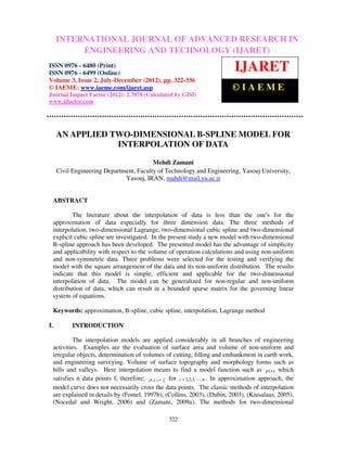
Fairs, 2010). For a problem with a set of 9 triple data A ε {(xi, yi, zi) i=1,2,…,9)} Figure 1.
The two-dimensional Lagrange equation is as follows,

( x − x 2 )( x − x3 )( y − y 4 )( y − y 7 ) ( x − x1 )( x − x3 )( y − y 4 )( y − y 7 )
z ( x, y ) = z1 + z2 +
( x1 − x 2 )( x1 − x3 )( y1 − y 4 )( y1 − y 7 ) ( x2 − x1 )( x 2 − x3 )( y 2 − y 4 )( y 2 − y 7 ) (1)
( x − x1 )( x − x2 )( y − y 4 )( y − y 7 )
z3 + ( ) z 4 + L + ( ) z9
( x3 − x1 )( x3 − x2 )( y3 − y 4 )( y 3 − y 7 )

y

x

Fig: 1 Simple data distribution

The two-dimensional Lagrange model is limited in terms of applicability. The degree and
order of the Lagrange polynomial increases as the number of data point increases. Therefore,
it results in the oscillation and sinus behavior of the governing curve. Hence, the Lagrange
curves give high inclination and deviations from the real curves for the points between the
data or nodes. Therefore, the model is not applicable and efficient for huge engineering data.

1.2 B-spline Approximation Method
B-spline methods have been extended since 1970s. The designated B stands for Basis,
so the full name of this approach is the basic spline. B-spline methods are mostly used for
curves and surfaces in computer graphics. The 2nd and 3rd degree B-splines which are used
extensively for approximation of data are less applicable for the interpolation of data. With
some modifications and corrections the B-spline models specially the second and third
degrees can be applied for interpolation of huge data, particularly for one-dimensional
interpolation problems. The 2nd and 3rd degrees B-spline polynomials can be used for
approximation of n control points ( pi , i = 0,1,2, L , n − 1) (Saxena and Sahay, 2005) and (Salomon,
2006) as,

323


 1 − 2 1  pi −1 
 
t 1  − 2 2 0  pi 
1
Pi (t ) = t 2
 i = 1,2, L , n − 2 (2)
2
1
 1 0  pi +1 
 

−1 3 − 3 1  pi −1 

1 3 −6 3 0  pi 
 
Pi (t ) = t 3 t2 t 1   = t  [B]{p} i = 1,2,L, n − 3 (3)
6 − 3 0 3 0  pi +1 
 
1 4 1 0  p i + 2 
 
The above B-spline curves will not cross through the control points but pass near them. The initial
and terminal points (q1 and q2) of the cubic B-spline curve which are joint points can be obtained
from Eq. (4).
1
q1 = [ pi −1 + 4 pi + pi +1 ]
6
1 (4)
q2 = [ pi + 4 pi +1 + pi + 2 ]
6
The two-dimensional cubic B-spline can be obtained from the product of Eq. (3) in two dimensions
as,

[
pi (t , u ) = t  [B]{pi } u  [B]{p j } ]
T
(5)

[ ]
p i (t , u ) = t  [B ] z i , j [B ] {u} =
T

− 1 3 − 3 1  z i −1, j −1 z i , j −1 z i +1, j −1 z i + 2, j −1   − 1 3 − 3 1  u 3 
  z i + 2, j  1  3 − 6 0  
1 3 −6 3 0  z i −1, j z i, j z i +1, j   4 u 2 
t 3 t2 t 1 
6 − 3 0 3

0  z i −1, j +1 z i , j +1 z i +1, j +1 z i + 2, j +1  6  − 3 3 3
 
1  u 
(6)
    
1 4 1 0  z i −1, j + 2
 zi, j +2 z i +1, j + 2 z i + 2, j + 2   1
 0 0 0  1 
 

Where t , u ∈ [0,1] . Using the linear transformation from t and u to x and y; respectively for the
uniform B-spline surface patch in Fig. (2), the graph equation pi ( x, y) results as follows,

pi ( x, y ) = x [ A][B ][Z ][B ] [ A'] {y}
T T
(7)

where x  = x 2 x 1 ,  y  = y 2 y 1 and

 a2 0 0  a '2 2 a ' b ' b '2 
    1 x1
A =  2 ab a 0 , A'T =  0 a' b'  , a = , b=− ,
x2 − x1 x2 − x1
 b2 b 1 0 0 1 (8)
   
1 y1
a' = , b' = −
y 2 − y1 y 2 − y1

324


y

x

Fig: 2 Data distribution for B-spline surface patch

A network of data with (m+1)×(n+1) control points P00 through Pmn has (m+1) rows and
(n+1) columns with uniform x and y increments (∆x, ∆y ) . From the above network about (m-
2)×(n-2) local cubic B-spline graphs or patches can be obtained which have continuity at least
c1 on each element side. The final graph which consists of local graphs passes (m-1)×(n-1)
internal points qij . If the data points transfer to those internal joint points qij the final graph
would be a two-dimensional cubic B-spline which is obtained by the interpolation method.
Hence, the final graph crosses all the data points. For the details of this method, the situation
of internal joint points, and their coordinates refer to (Salomon, 2006). The qij can be
determined with respect to z value as Eq. (8).
1
qij =
36
[
( zi −1, j −1 + 4 z i , j −1+ zi +1, j −1 ) + 4( zi −1, j + 4 z i , j + zi +1, j ) + ( zi −1, j +1 + 4 z i , j +1+ zi +1, j +1 ) ] (8)

The interpolation by two-dimensional cubic B-spline of a network data with mesh m×n and
uniform ∆x and ∆y requires 2(m+n+2) more equations in order to satisfy the uniqueness of
the governing system of equations. However, it relates to the degree of polynomial B-spline
considered. The above extra equations should be obtained by satisfying the boundary
conditions. The governed linear system of equations is a kind of nonadigonal system. It is
clear that this model is not practical for problems having huge data points.

1.3 Two-dimensional Cubic Spline Method
This method is obtained by the product of two cubic spline equations in directions x and y as
Eq. (9).

s ij ( x, y ) = aij + bij ( x − x i ) + cij ( y − y j ) + d ij ( x − x i ) 2 + eij ( x − x i )( y − y j ) + f ij ( y − y j ) 2
+ g ij ( x − x i ) 2 ( y − y j ) + hij ( x − x i )( y − y j ) 2 + iij ( x − x i ) 3 ( y − y j ) + jij ( x − x i )( y − y j ) 3
(9)
+ k ij ( x − x i ) 2 ( y − y j ) 2 + lij ( x − x i ) 3 ( y − y j ) 2 + mij ( x − x i ) 2 ( y − y j ) 3
+ nij ( x − x i ) 3 ( y − y j ) 3 + oij ( x − x i ) 3 + pij ( y − y j ) 3

Where sij is bicubic spline which defines for each rectangular element and has 16 parameters.
Those parameters are obtained by satisfying the following 16 continuity equations on the
corners of each element.

325


sij ( xi , y j ) = f ij ⇒1 sij ( xi ±1 , y j ±1 ) = f i +1, j +1 ⇒ 3
∂sij ∂ 2 sij
( xi , y j ) ⇒ 3 ( xi , y j ) ⇒ 3 (10)
∂x ∂x 2
2
∂sij ∂ sij
( xi , y j ) ⇒ 3 ( xi , y j ) ⇒ 3
∂y ∂y 2
The above 16 equations of continuity for each element are written and combined together to
form a nonadiagonal linear system of equations. By adding the governing boundary
conditions to the above linear system it is complemented to a linear system of equations
which has a unique solution. This method of solution gives the c2 continuity along each node
and at least c1 continuity at the element sides.

1.4 Explicit Two-dimensional Cubic Spline Method
An explicit two-dimensional interpolation model has been developed by (Zamani, 2010) that
is the simplification of the above two-dimensional cubic spline method. He applied uniform
network of data set (rectangular distribution). The interpolation equation which is
implemented in his model is as follows,

sij ( x, y ) = a 0 + a1 ( x − x i ) + a 2 ( y − y j ) + a3 ( x − x i ) 2 + a 4 ( x − x i )( y − y j ) + a 5 ( y − y j ) 2
+ g ij ( x − x i ) 2 ( y − y j ) + a 6 ( x − x i ) 3 + a 7 ( x − x i ) 2 ( y − y j ) + a8 ( x − x i )( y − y j ) 2 (11)

+ a9 ( y − y j ) 3
The coefficients a0 to a9 are obtained by using c1 continuity on each element sides. They
consist of 4 equations of continuity for function and 6 equations of continuity for the first
partial derivatives along the x and y axis at 4 nodes of each element, Eqs. (12) and (13).

 sij ( xi , y j ) = f ij
 s (x , y ) = f
 ij i +1 j i +1, j
 (12)
 sij ( xi , y j +1 ) = f i , j +1
sij ( xi +1 , y j +1 ) = f i +1, j +1


 ∂ sij (i, j )  ∂ sij (i + 1, j )
 = f x',i , j  = f x',i +1, j
 ∂x  ∂x
 ∂ sij (i, j )  ∂ sij (i + 1, j )
 = f y' ,i , j  = f y' ,i +1, j (13)
 ∂y  ∂y
 ∂ sij (i, j + 1)  ∂ sij (i , j + 1)
 = f x',i , j +1  = f y' ,i , j +1
 ∂x  ∂y

With having the above partial derivatives the problem is unique and it consists of 10
equations and 10 unknowns which can be solved explicitly (it’s not necessary to form any
linear system of equations). In most cases the partial derivatives are not available at each

326


node but can be removed or eliminated by using numerical derivatives approaches. The
coefficients a0 to a9 of Eq. (11) can be determined from the following equations.

a0 = f ij , a1 = f x',ij , a2 = f y' ,ij ,

3 2 3 1
a3 = − a0 − a1 + 2 f i +1, j − f x',i +1, j (14)
hi2 hi hi hi

1 1 1 1 1 1 '
a4 = − a0 − a1 + ( f i +1, j + f i , j +1 − f i +1, j +1 ) + f y' ,i +1, j − a2 + f x ,i , j +1
hi k j kj hi k j hi hi kj

3 2 3 1 '
a5 = − a − a 2 + 2 f i , j +1 −
2 0
f y ,i , j +1
kj kj kj kj
2 1 2 1
a6 = a + 2 a1 − 3 f i +1, j + 2 f x',i +1, j
3 0
hi hi hi hi
1 1 1 1
a7 = 2
a0 + a1 − 2 ( f i +1, j + f i , j +1 − f i +1, j +1 ) − f x',i , j +1
h kj
i hi k j hi k j hi k j

1 1 1 1
a8 = a +
2 0
a2 − 2
( f i +1, j + f i , j +1 − f i +1, j +1 ) − f y' ,i +1, j
hi k j hi k j hi k j hi k j
2 1 2 1 '
a9 = 3 a0 + 2 a 2 − 3 f i , j +1 + 2 f y ,i , j +1
kj kj kj kj

Where hi and ki are length and width of element ij ; respectively. For a huge set of data
which usually exists in engineering problems the above model is simple and requires less
calculation operations with respect to the other methods of two-dimensional interpolation.
The only limitation for this model is determining the partial derivatives with respect to x and
y axis at each node and they should be approximated by the governing methods.

II. MODEL FORMULATION

The model is the generation of B-spline method in two dimensional, therefore; it is
better to explain a brief review of the one-dimensional B-spline.

2.1 One-dimensional B-spline
This model is explained in more detail by (Salamon, 2006) but in this study it is briefly
discussed. The B-spline curve consists of a series of B-spline basic functions that are linearly
independent in domain [a, b] as,
n
s ( x ) = ∑ ci β i [ui ( x )] =c 0 β 0 (u ) + c1 β1 (u ) + L + c n β n (u ) (15)
i =1

where u ∈ [−2,2] , u i ( x) = ( x − xi ) / h , h = (b − a ) / n and n is the number of elements. Each B-
spline basic function consists of four cubic polynomial functions as Eqs. (16).

327

July December

 (2 + u) 3 , − 2 ≤ u ≤ −1
 2 3
1 + 3(1 + u ) + 3(1 + u ) − 3(1 + u ) , −1 ≤ u ≤ 0

β i (u ) = 1 + 3(1 − u ) + 3(1 − u ) 2 − 3(1 − u )3 , 0 ≤ u ≤1
 (16)
(2 − u )3 , 1≤ u ≤ 2


 0 , otherwise

The following basic equation is applied for B-spline basic function for increasing its
B spline
applicability and continuity order (Zamani, 2009b).
 x − xi 2
−b  
−b u 2  h  (17)
β i (u ) = ae − c = ae −c

Where a = 4.016478 , b = 1 .3740615 and c = 0.016478 . Fig. (3) shows the B-spline basic
B
function for Eq. (17).

Fig: 3 B-spline basic function

In order to promote the accuracy and efficiency of B-spline method two basic functions
B spline
c−1 β −1 (u ) and cn+1 β n +1 (u ) are added to Eq. (15) for adding the effects of boundary conditions.
The coefficients c−1 and cn +1 can be calculated with respect to the B-spline curve at boundary
B spline
points according to the following equations.

c−1β −1 ( x ) + 4c0 β 0 ( x ) + c1β1 ( x ) = f (x ) (18)

c −1 β −1 ( x0 ) + 4c0 β 0' ( x0 ) + c1 β 1' ( x0 ) = f ' ( x0 )
' (19)

B-spline basic functions β −1 ( x ) , β 0 ( x) and β1 ( x) in Eq.
After making derivatives from the B
(19) it can be written as,

328


− c−1α + c1α = f ' ( x0 ) = f 0' (20)
' ' b
f f he
0 0
c−1 = c1 −
= c1 − (21)
α 2ab
h
where α = . In the same way the coefficient cn+1 for the last boundary point can be
2abe −h
obtained.
f n' f n' h e b
cn +1 = cn −1 + = cn −1 + (22)
α 2ab
With regarding to f 0' and f n' the derivatives at the first and the last points are not available
and should be approximated. This model gives a tridiagonal linear system of equations with
dimensions (n+1) × (n+1) with 4 on the main diagonal entries and 1 on the sub diagonal and
sup diagonal components. The obtained linear system of equations is easy to solve. This can
be done by Thomas algorithm. The above model results in smooth curves for data of having
nonlinear distributions and uniform elements. The model can also be extended for data of
non-uniform element length.

2.2 Two-dimensional B-spline
The two-dimensional B-spline model is the generation of one-dimensional model in two
directions and in cylindrical coordinates is as follows,
ρ2
−b
β k ( x, y ) = a e l2 h2
−c (23)

−
b
l2 h2
[( x− x ) +( y− y ) ]
i
2
j
2
(24)
β k ( x, y) = a e −c
where k is number of node having (xi, yi) coordinates. Eq. (24) for l = 2 / 2 is,

−
2b
h2
[( x − x )
i
2
+( y − y j ) 2 ] (25)
β ij ( x, y ) = a e −c
Where h is element length. The two-dimensional B-spline Eq. (25) for h=1 and ρ = 2 ,
2 / 2 and 0 equal 0, 1 and 4; respectively. The effective radius for B-spline function of Eq.
(25) is 2 . Figs. (4) and (5) show the graph of Eq. (25) and its contour line.

Fig: 4 Two-dimensional B-spline basic function graph

329

July December

Fig: 5 Two-dimensional B-spline basic function contour
dimensional B
Suppose there exist n data points with uniform rectangular or square mesh. The element dimensions
are constant all over the mesh with length h = hi = xi +1 − xi and k = k j = y j +1 − y j . The two-
dimension B-spline function for this set of data can be written as,
spline
n
s ( x, y ) = ∑ cm β m ( x, y ) = c1β1 + c3 β 3 + c3 β 3 + L cn β n (26)
m =1
where n is the total number nodes and m is the node number. For simplification of the formulation
let’s consider square elements with h = k = 1 . The B-spline function s ( x, y ) for node m is,

s ( xm , y m ) = f m ,m = cm − k β m − k + cm −1 β m −1 + cm β m + cm +1β m +1 + cm + k β m + k (27)

The values of B-spline basic functions from Eq. (27) equal,

β m − k = β m −1 = β m +1 = β m + k = α = a e −2b
 (28)
 βm = 4
If Eq. (27) is applied on each node the following linear system of equations Eq. (29) will be

4 α 0 0 0 α O 0   c1   f1 
α
 4 α O O O α O  c2   f 2 
   
0 α 4 α α  M   M 
    
0 O α 4 α O     (29)
0   =  = [ A] {c} = { f }
O α 4 α O    
 
α O α 4 α O  M   M 
O    
α α 4 α  cn −1   f n −1 
 

O O α O O O α 4   cn   f n 
   

obtained where it is pentadiagonal system with 4 on the main diagonal entries and α on the four others
diagonal components. Since the values of diagonal entries are constant, therefore; it is only necessary
to save the values of 4, α and their addresses to save matrix A. This saves computer memory
especially for problems with huge number of data.
Three problems are chosen for investigation of checking and efficiency of the above formulation
above
which are explained here.

330


2.2.1 Problem 1
There are 25 data points {xi , yi , z i ; i = 1,2,L,25} in this problem. They form a mesh point with
5 rows and 5 columns and square elements as Fig. (6). The element side is h = k = 1 . The
domain of function f ( x, y ) is x ∈ [0,4] , y ∈ [0,4] . The data are obtained from Eq. (30).

z = f ( x, y ) = e [0.71( x −1) ]0.5
2
+1.13 ( y − 2 ) 2 (30)

As indicated in Fig. (6) 20 auxiliary points or nodes around the data are considered for
including the effects of boundary conditions. This action causes an increase in accuracy and
efficiency of presented model for solving these kinds of problems.

Fig: 6 Data distribution in problem 1

Partial derivatives are required with respect to x axis and y axis at boundary nodes for this
purpose. For the most engineering data the above partial derivatives for boundary points are
not available and should be somehow approximated. The B-spline model which is used for
this problem is,
25 20
s ( x, y ) = ∑ ci β i ( x, y ) + ∑ cib β ib ( x, y ) (31)
i =1 i =1

In Eq. (31) the second set of equation is related to the effects of boundary conditions which
can be expanded as Eq. (32).
20

∑c
i =1
ib β ib ( x, y ) = c−1 y β −1 y + c− 2 y β − 2 y + L + c−5 y β −5 y +

c21 y β 21 y + c22 y β 22 y + L + c25 y β 25 y +
(32)
c−1 x β −1 x + c− 2 x β − 2 x + L + c− 21 x β − 21 x +
c5 x β 5 x + c6 x β 6 x + L + c25 x β 25 x

For calculation s( x, y ) or z value for internal points in each element it is necessary to consider
only a few terms of Eq. (31). Most of its terms are zero for each point inside the elements

331


because of the nature of B-spline basic function. Fig. (7) shows the amount of the
effectiveness with regard to the number of B-spline basic functions which contributes to
determining s ( x, y ) . For example in elements with nodes 8, 9, 13, and 14 the number of
required B-spline basic functions for calculation s ( x, y ) are from minimum 4 to maximum 7
Fig. (7). This problem is solved by the presented model. Figs. (8), (8a), (9) and (9a) show
the comparative behavior between the model and the real values of f ( x, y ) function for the
central points of elements. As it can be seen from the figures there are a suitable relationship
and agreements between the model output and the real data.

Fig: 7 Required number of B-spline basic function

4

3

y 2

1

0
0 1 2 3 4
x

0 0. 1 1. 2
Fig: 8 Graph of real data Fig: 8a Contour lines of real data

332

July December

4

3

y 2

1

0
0 1 2 3 4
x

Fig: 9 Graph of B-spline model
spline Fig: 9a Contour lines of B-spline model
B spline

2.2.2 Problem 2
This problem in relation to the previous one has more complexity with respect to the
variations of data. In this example there are 121 data points {xi , yi , zi ; i = 1,2,L,121}. The data
form a uniform mesh having 11 rows and 11 columns with the domain of function f ( x, y )
x ∈ [1,6] , y ∈ [1,6] . The data are generated by the following equation.

2 2 ( y − 4)π (33)
f ( x, y ) = [10 e −( x − 4.5) + 6.817 e −1.2( x − 2.5) ] Cos 2.53
8
About 44 auxiliary boundary nodes for applying the effects of boundary conditions are
considered. The partial derivatives with respect to x and y axis at boundary points are
calculated by the forward and backward divided difference formulas. The graph and contour
lines for Eq. (33) are in Figs. (10) and (10a). They are shown from the B-spline model in
s. B spline
Figs. (11) and (11a) as well. Comparison of the figures shows a good agreement and suitable
relationship between the real data and the interpolated data.
middle points f(x,y)

Fig: 10 Graph of real data Fig: 10a Contour lines of real data

333

July December

Fig: 11 Graph of B-spline model
spline Fig: 11a Contour lines of B-spline model
B spline

2.2.3 Problem 3
This example consists of 49 triple data points {xi , y i , z i ; i = 1,2,L,49} . According to Fig. (12),
they form a uniform square mesh with 7 rows and 7 columns of data and 36 elements with
element size h = k = 1.0 . The data which are highly nonlinear are obtained from Eq. (34).

z = ( x 2 + y 2 )Sin [8 Arctg ( x / y )] (34)

About 28 auxiliary points are considered for including the effects of boundary conditions.

43y +44 +45 +46 +47 +48 +49y

-43x 43 44 45 46 47 48 49 +49x
-36 36 37 38 39 40 41 42 +42
-29 29 30 31 32 33 34 35 +35
-22 22 23 24 25 26 27 28 +28
-15 15 16 17 18 19 20 21 +21
-8 8 9 10 11 12 13 14 +14
-1x 1 2 3 4 5 6 7 +7y

-1y -2
1y -3 -4 -5 -6 -7y
Fig: 12 Network of data and boundary points

The domain of data for this problem is x ∈ [1,7] , y ∈ [1,7] . Similar to the previous problem
the partial derivatives with respect to x axis and y axis at the boundary points are calculated
by the numerical method differentiation. The parameters governing to the boundary points
can be obtained from the above deri
derivatives. The parameters c7 x and c −7 y for example can be
determined from Eqs. (35) and (36).

334


1 '
c7 x = c6 + f x (7 ) (35)
A
1
c− 7 y = c14 − f y' (7) (36)
A
where A = 8abe −b . The two dimensional B-spline basic function which is applied for this problem
for h = 1.0 and l = 2 / 2 is,

β k ( x, y ) = a e
[
−2 b ( x − xi ) 2 + ( y − y j ) 2 ]−c (37)

The graphs and contour lines obtained by the model and from the function f ( x, y ) are in Figs. (13),
(13a), (14) and (14a). A comparison between these figures presents a good and suitable relationship
for real data and the two-dimensional B-spline model.

f(x,y)
f(x,y)

6.5

6

5.5

5

4.5

y 4

3.5

3

2.5

2

1.5
1.5 2 2.5 3 3.5 4 4.5 5 5.5 6 6.5
Fig: 13 Graph of real data
x Fig: 13a. Contour lines of real data

B-spline model B-spline model

6.5

6

5.5

5

4.5

y 4

3.5

3

2.5

2

1.5
1.5 2 2.5 3 3.5 4 4.5 5 5.5 6 6.5
x

Fig: 14 Graph of B-spline model Fig: 14a Contour lines of B-spline model

335


III. CONCLUSIONS AND DISCUSSION

The interpolation methods especially the two-dimensional ones have many
applications in all branches of engineering science. Therefore; the development, extension
and improvement of these methods are necessary. The presented model is easy to implement
and results in a linear pentadiagonal systems of equations which is diagonally dominant and
simply solvable. The presented model for interpolation of data with rectangular and square
elements is powerful. Also it can be expanded for non-uniform mesh or triangular elements
of data. The final linear system of equations for those cases is sparse and bounded while
about more than 90% of matrix entries are zero. The graphs obtained by this method have no
limitations of continuity properties inside and across the elements because of the continuity
conditions of the applied B-spline basic function. These conditions explain the advantage
and robustness of the presented model to the available methods of two-dimensional
interpolation.

REFERENCES

Burden, R. and Fairs, J. (2010). Numerical Analysis, 9th Ed. Brooks-Cole Pub.
Comp.Boston.
Collins, G. W. (2003). II Fundamental Numerical Methods and Data Analysis, (internet pdf
file).
Dierckx, P. (1993.) Curve and Surface Fitting with splines, Clarendon Press, NY.
Dubin, D. (2003). Numerical and Analytical Methods for Scientists and Engineers Using
Mathematica, John Wiley & Sons, Inc., Pub., Hokoben, New Jersy.
Fomel, S. (1997b). On the General Theory of Data Interpolation, SEP. 94, 165-179.
Kiusalaas, J. (2005). Numerical Methods In Engineering with MATLAB, Cambridge Univ.
Press,UK.
Lobo, N. (1995). Curve fitting using spline sections of different orders, Proceedings of the
First International Mathematics Symposium, P. 267-274.
Nocedal, J. and Wright, S. J. (2006). Numerical Optimization, 2nd Ed., Springer, Science
+Business Media, LLC, USA.
Salomon, D. (2006). Curves and Surfaces for computer Graphics, Springer Science
+Business Media, Inc. USA.
Saxena, A. and Sahay B. (2005). Computer Aided Engineering Design, Springer, Anamaya
Publishers, New Delhi, India.
Zamani, M. (2009 a). Three simple spline methods for approximation and interpolation of
data, Contemporary Engineering Science, Vol.2, No.8, P. 373-381.
Zamani, M. (2009 b). An investigation of B-spline and Bezier methods for interpolation of
data, Contemporary Engineering Science, Vol.2, No.8, P. 361-371.
Zamani, M. (2010). A simple 2-D interpolation model for analysis of nonlinear data, Natural
Science, Vol. 2, No. 6, June 2010, P. 641-646.
M. Nagaraju Naik and P. Rajesh Kumar, “Spectral Approach To Image Projection With
Cubic B-Spline Interpolation” International journal of Electronics and Communication
Engineering &Technology (IJECET), Volume3, Issue3, 2012, pp. 153 - 161, Published by
IAEME

336

An applied two dimensional b-spline model for interpolation of data

Recommended

Recommended

More Related Content

What's hot

What's hot (20)

Viewers also liked

Viewers also liked (6)

Similar to An applied two dimensional b-spline model for interpolation of data

Similar to An applied two dimensional b-spline model for interpolation of data (20)

More from iaemedu

More from iaemedu (20)

An applied two dimensional b-spline model for interpolation of data