Chapter10

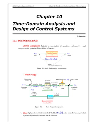
ME 413 Systems Dynamics & Control Chapter 10: Time-Domain Analysis and Design of Control Systems
1/11
Chapter 10
Time-Domain Analysis and
Design of Control Systems
A. Bazoune
10.1 INTRODUCTION
Block Diagram: Pictorial representation of functions performed by each
component of a system and that of flow of signals.
( )C s( )R s
( ) ( ) ( )=C s G s R s
Figure 10-1. Single block diagram representation.
Terminology:
( )C s( )R s ( )G s1 ( )G s2
( )H s
( )Disturbance U s
± ( ) ( ) ( )E s R s b s= ± ( )M s
( )B s
Figure 10-2. Block Diagram Components.
1. Plant: A physical object to be controlled. The Plant ( )G s2 , is the controlled system, of which
a particular quantity or condition is to be controlled.

2/11
2. Feedback Control System: A system which compares output to some reference input and
keeps output as close as possible to this reference.
3. Closed-loop Control System: same as feedback control system.
4. Open-loop Control System: Output of the system is not feedback to the system.
5. The Control Elements ( )G s1
, also called the controller, are the components required to
generate the appropriate control signal ( )M s applied to the plant.
6. The Feedback Elements ( )H s is the components required to establish the functional
relationship between the primary feedback signal ( )B s and the controlled output ( )C s .
7. The Reference Input ( )R s is an external signal applied to a feedback control system in order
to command a specified action of the plant. It often represents ideal plant output behavior.
8. The Controlled Output ( )C s is that quantity or condition of the plant which is controlled.
9. The Primary Feedback signal ( )B s is a signal which is a function of the controlled output
( )C s , and which is algebraically summed with the reference input ( )R s to obtain the
actuating signal ( )E s .
10. The Actuating Signal ( )E s , also called the error or control action, is the algebraic sum
consisting of the reference input ( )R s plus or minus (usually minus) the primary feedback
( )B s .
11. The Manipulated Variable ( )M s (control signal) is that quantity or condition which the
control elements ( )G s1
apply to the plant ( )G s2
.
12. A Disturbance ( )U s is an undesired input signal which affects the value of the controlled
output ( )C s . It may enter the plant by summation with ( )M s , or via an intermediate
point, as shown in the block diagram of the figure above.
13. The Forward Path is the transmission path from the actuating signal e to the controlled output
( )C s .
14. The Feedback Path is the transmission path from the controlled output ( )C s to the primary
feedback signal ( )B s .
15. Summing Point: A circle with a cross is the symbol that indicates a summing point. The ( )+
or ( )− sign at each arrowhead indicates whether that signal is to be added or subtracted.
16. Branch Point: A branch point is a point from which the signal from a block goes concurrently
to other blocks or summing points.

3/11
10.2 BLOCK DIAGRAMS AND THEIR SIMPLIFICATION
Definitions:
( )C s( )R s ( )G s
( )H s
( )B s
( )E s
Figure 10-3 Block diagram of a closed-loop system with a feedback element.
1. ( )G s ≡Direct transfer function = Forward transfer function
2. ( )H s ≡Feedback transfer function
3. ( ) ( )G s H s ≡ Open-loop transfer function
4. ( ) ( )C s R s ≡ Closed-loop transfer function = Control ratio
5. ( ) ( )C s E s ≡Feedforward transfer function
Closed Loop Transfer Function:
For the system shown in Figure 10-3, the output ( )C s and input ( )R s are related as follows:
( ) ( ) ( )=C s G s E s
where
( ) ( ) ( ) ( ) ( ) ( )= − = −E s R s B s R s H s C s
Eliminating ( )E s from these equations gives
( ) ( ) ( ) ( ) ( )[ ]= −C s G s R s H s C s
This can be written in the form
( ) ( )[ ] ( ) ( ) ( )+ =G s H s C s G s R s1
or
( )
( )
( )
( ) ( )
=
+
C s G s
R s G s H s1
The Characteristic equation of the system is defined as an equation obtained by setting the
denominator polynomial of the transfer function to zero. The Characteristic equation for the above
system is ( ) ( )G s H s+ =1 0.

4/11
Block Diagram Reduction Rules
In many practical situations, the block diagram of a Single Input-Single Output (SISO),
feedback control system may involve several feedback loops and summing points. In
principle, the block diagram of (SISO) closed loop system, no matter how complicated it is, it
can be reduced to the standard single loop form shown in Figure 10-3. The basic approach to
simplify a block diagram can be summarized in Table 1:
TABLE 10-1 Block Diagram Reduction Rules
1 Combine all cascade blocks
2 Combine all parallel blocks
3 Eliminate all minor (interior) feedback loops
4 Shift summing points to left
5 Shift takeoff points to the right
6 Repeat Steps 1 to 5 until the canonical form is obtained
TABLE 10-2. Some Basic Rules with Block Diagram Transformation
G1u
2u
y
1/G
1u
1
y G u
u y
G
=
=
y Gu=
Gu
u
y
( )2 1 2e G u u= −
Gu
y
y
G
G1u
2u
y
G1u
2u
y
G
u
y
y
G
u
y
1/G
Gu
G
2u
y 1 2y Gu u= −
u ( )1 2y G G u= −1G y21/G2G
( )Y GG X= 1 21G Y2GX
( )Y G G X= ±1 2
1G
2G
X
Y±±±±
1 2G GX Y
1 2±G GX Y

5/11
█ Example 1
A feedback system is transformed into a unity feedback system

6/11
=
±
⋅=
±
=
GH
GH
HGH
G
R
C
1
1
1
Closed-loop Transfer function
█ Example 2
Let us reduce the following block diagram to canonical form.
⇒⇒⇒⇒
⇒⇒⇒⇒
⇒⇒⇒⇒
Step 4:
⇒⇒⇒⇒
█ Example 3

7/11

8/11
█ Example 4
Use block diagram reduction to simplify the block diagram below into a single block relating
( )Y s to ( )R s .
█ Solution

9/11
█ Example 5
Use block diagram algebra to solve the previous example.
█ Solution
Multiple-Inputs cases
In feedback control system, we often encounter multiple inputs (or even multiple output
cases). For a linear system, we can apply the superposition principle to solve this type of
problems, i.e. to treat each input one at a time while setting all other inputs to zeros, and then
algebraically add all the outputs as follows:
TABLE 10-3: Procedure For reducing Multiple Input Blocks
1 Set all inputs except one equal to zero
2 Transform the block diagram to solvable form.
3 Find the output response due to the chosen input action alone
4 Repeat Steps 1 to 3 for each of the remaining inputs.
5 Algebraically sum all the output responses found in Steps 1 to 5

10/11
█ Example 6
We shall determine the output C of the following system:
█ Solution
Step1: Put 0≡U
Step2: The system reduces to
Step 3: The output RC due to input R is R
GG
GG
CR ⋅
+
=
21
21
1
Step 4a: Put R = 0.
Step 4b: Put -1 into a block, representing the negative feedback effect:
Rearrange the block diagram:
Let the -1 block be absorbed into the, summing point:
Step 4c: By Equation (7.3), the output UC due to input U is U
GG
G
CU ⋅
+
=
21
2
1
Step 5: The total output is C:

11/11
[ ]URG
GG
G
U
GG
G
R
GG
GG
CCC UR +⋅
+
=⋅
+
+⋅
+
=+= 1
21
2
21
2
21
21
111
█ Example 7

1/10
Chapter 10
Time-Domain Analysis and Design of
Control Systems
A. Bazoune
10.5 TRANSIENT RESPONSE SPECIFICATIONS
Because systems that stores energy cannot respond instantaneously, they exhibit a transient
response when they are subjected to inputs or disturbances. Consequently, the transient
response characteristics constitute one of the most important factors in system design.
In many practical cases, the desired performance characteristics of control systems can
be given in terms of transient-response specifications. Frequently, such performance
characteristics are specified in terms of the transient response to unit-step input, since such an
input is easy to generate and is sufficiently drastic. (If the response of a linear system to a step
input is known, it is mathematically possible to compute the system’s response to any input).
The transient response of a system to a unit step-input depends on initial conditions.
For convenience in comparing the transient responses of various systems, it is common
practice to use standard initial conditions: The system is at rest initially, with its output and
all time derivatives thereof zero. Then the response characteristics can be easily compared.
Transient-Response Specifications. The transient response of a
practical control system often exhibits damped oscillations before reaching a steady state. In
specifying the transient-response characteristics of a control system to a unit-step input, it is
common to name the following:

2/10
1. Delay time, dT
2. Rise time, rT
3. Peak time, pT
4. Maximum overshoot, pM
5. Settling time, sT
These specifications are defined next and are shown in graphically in Figure 10-21.
Delay Time. The delay time dT is the time needed for the response to reach half of
its final value the very first time.
Rise Time. The rise time rT is the time required for the response to rise from 10%
to 90%, 5% to 95%, or 0% to 100% of its final value. For underdamped second order systems,
the 0% to 100% rise time is normally used. For overdamped systems, the 10% to 90% rise time
is common.
Peak Time. The peak time pT is the time required for the response to reach the first
peak of the overshoot.
Maximum (percent Overshoot). The maximum percent overshoot pM is the
maximum peak value of the response curve [the curve of ( )c t versus t ], measured from
( )c ∞ . If ( ) 1c ∞ = , the maximum percent overshoot is 100%pM × . If the final steady state
value ( )c ∞ of the response differs from unity, then it is common practice to use the
following definition of the maximum percent overshoot:
( ) ( )
( )
100Maximum percent overshoot %
pC t C
C
− ∞
= ×
∞
Settling Time.The settling time sT is the time required for the response curve to reach
and stay within 2% of the final value. In some cases, 5%instead of 2%, is used as the
percentage of the final value. The settling time is the largest time constant of the system.
Comments. If we specify the values of dT , rT , pT , sT and pM , the shape of the
response curve is virtually fixed as shown in Figure 10.22.
Figure 10-22 Specifications of transient-response curve.

3/10
A Few Comments on Transient Response-Specifications.
In addition of requiring a dynamic system to be stable, i.e., its response does not increase
unbounded with time (a condition that is satisfied for a second order system provided that
0ζ ≥ , we also require the response:
• to be fast
• does not excessively overshoot the desired value (i.e., relatively stable) and
• to reach and remain close to the desired reference value in the minimum time
possible.
Second-Order Systems and Transient-Response-Specifications.
The response for a unit step input of an underdamped second order system ( )0 1ζ< < is
given by
( ) 2
2
1 sin cos
1
1 sin cos
1
ζω ζω
ζω
ζ
ω ω
ζ
ζ
ω ω
ζ
− −
−
= − −
−
= − +
−
  
 
  
n n
n
t t
d d
t
d d
c t e t e t
e t t
(10-13)
or
( )
2
1
2
1
1 sin tan
1
ζω
ζ
ω
ζζ
−
− −
= − +
−
  
 
  
n
t
d
e
c t t (10-14)
A family of curves ( )c t plotted against t with various values of ζ is shown in Figure 10-24.
2
2 2
2
n
n ns s
ω
ζ ω ω+ +
− − − − −
Input
t
( )u t
1
0 2 4 6 8 10 12 14 16 18 20
0
0.2
0.4
0.6
0.8
1
1.2
1.4
1.6
Step Response
Time (sec)
Amplitude
ζ = 0.2
0.5
0.7
1
2
5
Output
_______________
Figure 10-24 Unit step response curves for a second order system.

4/10
Delay Time. We define the delay time by the following approximate
formula:
1 0 7.
d
n
T
ζ
ω
+
=
Rise Time. We find the rise time rT by letting ( ) 1rc T = in Equation (10-13), or
( ) 2
1 1 sin cos
1
ζω ζ
ω ω
ζ
−
= = − +
−
  
 
  
n r
T
d dr r rc T e T T (10-15)
Since 0ζω−
≠n
t
e , Equation (10-15) yields
2
sin cos 0
1
ζ
ω ω
ζ
+ =
−
d dr rT T
or
2
1
tan
ζ
ω
ζ
−
= −d rT
Thus, the rise rT is
2
1 11
tan
ζ
ω ζ ω
π β− −
= −
  −
= 
 
 d d
rT (10-16)
where β is defined in Figure 10-25. Clearly to obtain a large value of rT we must have a
large value of β .
O
σ
S-plane
jω
nω
σ−
nζω
2
1nω ζ−
djω
β
( )
( )
1
1 2
2
1
cos
or sin 1
1
or tan
β ζ
β ζ
ζ
β
ζ
−
−
−
=
= −
 −
=  
 
 
Figure 10-25 Definition of angle β
Peak Time. We obtain the peak time pT by differentiating ( )c t in Equation (10-13),
with respect to time and letting this derivative equal zero. That is,

5/10
( )
2
sin 0
1
ζωω
ω
ζ
−
= =
−
n
tn
de
dc t
t
dt
It follows that
sin 0ω =dt
or
0, , 2 , 3 ,... , 0,1,2.....ω π π π π= = =dt n n
Since the peak time pT corresponds to the first peak overshoot ( )1n = , we have ω π=d pT .
Then
2
1
π π
ω ω ζ
= =
−
p
d n
T (10-17)
The peak time pT corresponds to one half-cycle of the frequency damped oscillations.
Maximum Overshoot pM The maximum overshoot pM occurs at the peak
π ω=p dT . Thus, from Equation (10-13),
( ) ( )
2
1
1
0
1
sin cos
n d
p pM c T e
ζω π ω ζ
π π
ζ
−
 
 
 
= −
− −
=
+ 
− 
  
= =
or
21
pM e πζ ζ− −
= (10-18)
Since ( ) 1c ∞ = , the maximum percent overshoot is
21
100% %pM e πζ ζ− −
×=
The relationship between the damping ratio ζ and the maximum percent overshoot is
shown in Figure 10-26. Notice that no overshoot for 1ζ ≥ and overshoot becomes negligible
for 0 7.ζ > .

6/10
Figure 10-26 Relationship between the maximum percent overshoot %pM and damping ratio ζ
Settling Time sT Based on 2%criterion the settling time sT is defined as:
( )
( ) 4
0 02
0 02
0 02
ln
ln
.
.
.n s s
n n
n sT
T T
e ζω
ζω
ζω ζω
−
− = = ≈
−
=
⇒
( )
4
2% Criterion
n
sT
ζω
= (10-19)
Similarly for 5%we can get
( )
3
5% Criterion
n
sT
ζω
= (10-20)

7/10
REVIEW AND SUMMARY
TRANSIENT RESPONSE SPECIFICATIONS OF A SECOND ORDER SYSTEM
TABLE 1. Useful Formulas and Step Response Specifications for the Linear
Second-Order Model )(tfxkxcxm =++ where m, c, k constants
1. Roots
m
mkcc
s
2
42
2,1
−±−
=
2. Damping ratio or mkc 2/=ζ
3. Undamped natural frequency
m
k
n =ω
4. Damped natural frequency 2
1 ζωω −= nd
5. Time constant ncm ζωτ /1/2 == if 1≤ζ
6. Logarithmic decrement
2
1
2
ζ
πζ
δ
−
= or
22
4 δπ
δ
ζ
+
=
7. Stability Property Stable if, and only if, both roots have negative real parts, this
occurs if and only if , m, c, and k have the same sign.
8. Maximum Percent Overshoot: The maximum % overshoot pM is the maximum peak
value of the response curve.
2
1/
100 ζπζ −−
= eM p
9. Peak time: Time needed for the response to reach the first peak of the overshoot
2
1/p nT π ω ζ= −
10. Delay time: Time needed for the response to reach 50% of its final value the first time
1 0 7.
d
n
T
ζ
ω
+
≈
11. Settling time: Time needed for the response curve to reach and stay within 2% of the final
value
4
s
n
T
ζω
=
12. Rise time: Time needed for the response to rise from (10% to 90%) or (0% to 100%) or (5% to
95%) of its final value r
d
T
π β
ω
−
= (See Figure 10-25)

8/10
SOLVED PROBLEMS
█ Example 1
Figure 4-20 (for Example 1)
█ Example 2

9/10
Figure 4-21 (for Example 2)
█ Solution
First The transfer function of the system is
█ Example 3 (Example 10-2in the Textbook Page 520-521)
Determine the values of dT , rT , pT , sT when the control system shown in Figure 10-28 is
subject to a unit step input

10/10
( )
1
1+s s
( )C s( )R s
Figure 10-28 Control System
█ Solution
The closed-loop transfer function of the system is
( )
( )
( )
( )
2
1
1 1
1 11
1
C s s s
R s s s
s s
+
= =
+ ++
+
Notice that 1nω = rad/s and 0 5.ζ = for this system. So
2 2
1 1 0 5 0 866. .d n
ω ω ζ= − = − =
Rise Time.
ω
π β−
=
d
rT
where
( ) ( )1 1
0 866 1 1 05sin sin . .d nβ ω ω− −
= = = rad
or
( ) ( ) ( )1 1 1
0 5
1 05
cos cos cos
d
.
ra.
n nβ ζω ω ζ− − −
= = =
=
Therfore,
1.05
2.41
0.866
π −
= =rT s
Peak Time. 3 63
0 866
.
.
p
d
T
π π
ω
= = = s
Delay Time.
( )1 0 7 0 51 0 7
1 35
1
. ..
.d
n
T
ζ
ω
++
= = = s
σ
jω
nω
σ−
nζω
2
1nω ζ−
djω
β
Maximum Overshoot :
1 81
2 21 0 5 1 0 5
0 163 16 3.. .
. . %pM e e eπζ ζ π −− − − × −
= = = ==
Settling time:
4 4
8
0 5 1.
s
n
T
ζω
= = =
×
s

ME 413 Systems Dynamics & Control Section 10-4: Stability
1/20
9 Chapter 10
Time Domain Analysis and Design of
Control System
A. Bazoune
10.7 STABILITY ANALYSIS
Stability Conditions Using Rolling Ball
The base of the hollow is in equilibrium point. If the ball is displaced a small distance
from this position and released, it oscillates but ultimately returns to its rest position
at the base as it loses energy as a result of friction. This is therefore a stable
equilibrium point. (With no energy dissipation the ball would roll back and forth forever
and exhibit neutral stability).
The ball is in equilibrium if placed exactly at the top of the surface, but if it is displaced
an infinitesimal distance to either side, the net gravitational force acting on it will cause
it to roll down the surface and never return to the equilibrium point. This equilibrium is
therefore unstable.
The ball neither moves away nor returns to its equilibrium position. The flat portion
represents a neutrally stable region.

2/20
Stability Analysis in the Complex Plane
The stability of a linear closed-loop system can be determined from the location of the
closed-loop poles in the s-plane. If any of these poles lie in the Right-Half of the s-plane
(RHS), then with increasing time, they give rise to the dominant mode, and the transient
response increases monotonically or oscillates with increasing amplitude. Either of these
motions represents an unstable motion.
Location of roots of characteristic equations and the corresponding impulse response
For such a system, as soon as the power is turned on, the output may increase with time.
If no saturation takes place in the system and no mechanical stop is provided, then the
system may eventually be damaged and fail, since the response of a real physical system
cannot increase indefinitely.
Stability may be defined as the ability of a system to restore its equilibrium position
when disturbed or a system which has a bounded response for a bounded output.
Consider a simple feedback system
( )C s( )E s( )R s
( )G s
( )H s
The overall transfer function is given by
( )
( )
( )
( ) ( )1
C s G s
R s G s H s
=
+
The denominator of the transfer function ( ) ( )1 G s H s+ is known as the characteristic
polynomial. The characteristic equation is of the above system is
( ) ( )1 0G s H s+ =
What are the roots of the characteristic equation?

3/20
Let us write the characteristic equation in the form:
( )
( )( )( ) ( )
( )( )( ) ( )
1 2 3
1 2 3
...
...
n
m
s z s z s z s z
T s
s p s p s p s p
− − − −
=
− − − −
where 1 1, ,..., nz z z are the zeros of ( )T s and 1 1, ,..., mp p p are the poles of ( )T s . If the
input ( )R s is given then
( ) ( ) ( )C s T s R s=
or
( )
( )( )( ) ( )
( )( )( ) ( )
( )( )( ) ( )
( )( )( ) ( )
1 2 3
1 2 3
......
... ...
i ii iii jn
m i ii iii k
s z s z s z s zs z s z s z s z
C s
s p s p s p s p s p s p s p s p
 − − − − − − − −  
=   
− − − − − − − −    
In order to compute the output, we resort the above equation into partial fraction
expansion
( )
( ) ( ) ( ) ( ) ( ) ( )
1 21 2
1 2
... ...
ijn i i
m i ii ik
KK K KK K
C s
s p s p s p s p s p s p
      
= + + + + + + +   
− − − − − −      
The first bracket contains time that originates from the system itself. Terms in the
first bracket will give rise to time in the form
1 2
1 2, ,..., np t p t p t
nK e K e K e
where p j tσ ω= + . The above expression can be rewritten as
1 21 2
1 2, ,..., nnj t j t j t
nK e e K e e K e eω ω ωσσ σ
Terms of the imaginary exponent are basically sinusoidal functions(which will never die
away). Terms with real exponent must have negative values in order to force the
sinusoidal functions to approach a very small magnitude (die away). The location of the
roots of the characteristic equation on the s-plane will indicate the condition of
stability.
Stable
region
Unstable
region
Im
Re
Margin
Stability
s-plane
s jσ ω= +

4/20
Routh Stability criterion
The characteristic equation of the simple feedback system can be written as
( ) ( ) ( ) 1 2
1 2 1 01 0n n n
n n nF s G s H s a s a s a s a s a− −
− −= + = + + + + + =
Two Necessary But Insufficient Conditions
There are two necessary but insufficient conditions for the roots of the characteristic
equation to lie in Left Hand Side (LHS)-plane (i.e., stable system)
1. All the coefficients 1 2 1, , ,... ,n n na a a a− − and 0a should have the same sign.
2. None of the coefficients vanish (All coefficients of the polynomial should exist).
█ Example 1 Given the characteristic equation,
( ) 6 5 4 3 2
24 3 4 4a s s s s s s s= + + + + +−
Is the system described by this characteristic equation stable?

5/20
█ Solution
One coefficient (-2) is negative. Therefore, the system does not satisfy the necessary
condition for stability.
█ Example 2 Given the characteristic equation,
( ) 6 5 4 2
4 3 4 4a s s s s s s= + + + + +
Is the system described by this characteristic equation stable?
█ Solution
The term
3
s is missing. Therefore, the system does not satisfy the necessary condition
for stability.
Necessary and Sufficient Condition
The necessary and sufficient condition for the roots of the characteristic equation to
lie in Left Hand Side (LHS)-plane (i.e., stable system) is
0 1 2 3Polynomial Hurwitz Determinant , , , ...kD k> = (4)
This criterion is an algebraic method that:
1. provides information on the absolute stability of a Linear Time Invariant (LTI)
system that has a characteristic equation with constant coefficients.
2. indicates whether any of the roots of the characteristic equation lie in (RHS)-
plane.
3. indicates the number of roots that lie on the jω -axis and gives the range of
some system parameters over which the system can be stable.
How to Apply the Test
Let us write the characteristic equation in the form:
( ) ( ) ( ) 1 2
1 2 1 01 0n n n
n n nF s G s H s a s a s a s a s a− −
− −= + = + + + + + =
Step 1: Arrange the coefficients of the above equation into two rows. The
first row consists of the first, third, fifth, …, coefficients. The
second row consists of the second, fourth, sixth,…, coefficients, all
counting from the highest term as shown in the tabulation below
na 2na − 4na − 6na −
1na − 3na − 5na − 7na −

6/20
Step 2: Form the following array of numbers by the indicated operations,
illustrated here for a sixth-order equation:
6 5 4 3 2
6 5 4 3 2 1 0 0a s a s a s a s a s a s a+ + + + + + =
6s
5s
4
s
3
s
2
s
1
s
0
s
6a 4a 2a 0a
5a 3a 1a 0
5 4 6 3
5
=
−
A
a a a a
a
5 2 6 1
5
=
−
B
a a a a
a 0
5 0 6
5
0
=
− ×
a
a a a
a
53
=
−
C
Aa a B
A
051
=
−
D
Aa a a
A
5
0
0 0
=
× − ×A a
A
=
−
E
BC AD
C
0
0
0
=
− ×
a
Ca A
C
0
0 0
=
× − ×C A
C
0
=
−
F
ED Ca
E
0 0
0
0
0
0
0
0
0
=
− ×
a
Fa E
F
0 0 0
The previous table can also be obtained as follows:

7/20
6s
5s
4
s
3
s
2
s
1
s
0
s
6a 4a 2a 0a
5a 3a 1a 0
6 4
5 3
5
=
−
A
a a
a a
a
6 2
5 1
5
=
−
B
a a
a a
a 0
6 0
5
5
0
=
−
a
a a
a
a
5 3
=
−
C
a a
A B
A
0
5 1
=
−
D
a a
A a
A
5
0
0
0
=
−
a
A
A
=
−
E
A C
B D
C
0
0
0
=
−
a
A C
a
C
0
0 0
=
−
A C
C
0
=
−
F
C E
D a
E
0 0
0
0
0
0
0
0
0
=
−
a
E F
a
F
0 0 0
█ Example 1 Given
( )
( )2
5 4 3 2
2 2 25
3 9 16 10
s s
H s
s s s s s
+ +
=
+ + + + +
Check whether this system is stable or not.
█ Solution
The characteristic equation is:
5 4 3 2
3 9 16 10 0s s s s s+ + + + + =
Construct the Routh array

8/20
5s 1 3 16 0
4s 1 9 10 0
3s
1 3 9 1
6
1
× − ×
= −
1 16 10 1
6
1
× − ×
= 0 0
2s
6 9 6 1
10
6
− × − ×
=
−
6 10 0 1
10
6
− × − ×
=
−
0 0
1s
( )10 6 10 6
12
10
× − × −
=
( )10 0 0 6
0
10
× − × −
= 0 0
0s
( )12 10 0 10
10
12
× − ×
= 0 0 0
There are 2 sign changes. There are 2 poles on the right half of the “s” plane.
Therefore, the system is unstable.
Pole-Zero Map
Real Axis
ImaginaryAxis
-1.5 -1 -0.5 0 0.5 1
-5
-4
-3
-2
-1
0
1
2
3
4
5
pzmap plot
█ Example 2 In the figure below, determine the range of K for the system to be
stable
( )C s( )E s( )R s
( )( )1 2
K
s s s+ +
█ Solution: The characteristic equation is:
( )( )
1 ( ) ( ) 1 0
1 2
+ = + =
+ +
K
G s H s
s s s
or ( )( ) 3 2
1 2 0 3 2 0+ + + = ⇒ + + + =s s s K s s s K

9/20
3s 1 2 0
2s 3 K 0
1s
2 3 1 6
3 3
K K× − × −
= 0 0
0s
6
3 0
3
6
3
K
K
K
K
− × − × 
  =
− 
 
 
0 0
For the system to be stable we must have the following two conditions satisfied
simultaneously:
i) 0>K
and
ii)
6
0 6 0 6
3
−
> ⇒ − > ⇒ <
K
K K
The above two conditions can be shown graphically on the real line
0 1 2 3 4 5 6−∞ +∞
0>K
6<K
0 6< <K
The intersection of the two conditions above gives the condition for the stability
of the above system, that is 0 6< <K . What will happen if 0=K or 6=K ?
For 0=K , the above characteristic equation becomes
3 2
3 2 0 0+ + + =s s s
or
( )


+ + = ⇒ = −
 = −
=

⇒
2
0 The system is marginally stable
3 2 0 1
2
s
s
s s s
s
For 6=K , the above characteristic equation becomes
3 2
3 2 6 0+ + + =s s s or ( ) ( )2
2 3 03 =+ + +s ss
or
( )( )
= −

+ = + ⇒
= − ⇒
+ = ⇒ 


2
3
3 2 0 s j
s
s j
s s

10/20
The frequency of oscillations in the previous case is 2 rad/s.
Special Cases
i) Zero Coefficient in the First Column of the Routh’s
Array
When the first term in a row is zero, the following element of (power-1) s will be
infinite. One of the following methods may be used.
1 Substitute for =
1
s
x
in the original equation The same
criterion applies for x . Then solve for x .
2 Multiply the original equation by ( )+s a , 1, 2,3,...,=a This
introduces an additional negative root. Then follow the same procedure to check for
stability.
3 Substitute a small parameter ε for the 0 . Complete the
array and take the limit as 0ε → .
█ Example 3
Check whether the following system given by its characteristic equation is stable
or not
( )Γ = + = + + + + =4 3 2
1 ( ) ( ) 2 2 5 0s G s H s s s s s
█ Solution
4s 1 2 5
3s 1 2 0
2s
1 2 1 2
0
1
× − ×
=
1 5 1 0
5
1
× − ×
=
1s
0s
Method 1: Substitute for
1
=s
x
in the original equation.
The above characteristic equation is:
Zero element in the first column,
we can’t continue as usual.

11/20
( ) 4 3 2
2 2 5 0Γ = + + + + =s s s s s
Substitute
1
=s
x
in the above
( ) ( ) ( ) ( ) ( )
4 3 2
1 1 2 1 2 1 5 0= + + + + =B x x x x x
or ( ) 4 3 2
5 2 2 1 0= + + + + =B x x x x x
4x 5 2 1
3x 2 1 0
2x 2 2 1 5 1
2 2
× − × −
= 1
1x
( )
( )
1 2 1 1 2
5
1 2
− × − ×
=
−
0
0x 1
There are two sign changes. Therefore, there are 2 roots that lie on the right half of the
s-plane. The system is unstable.
Method 2: Multiply by ( )+s a in the original equation.
Let 1=a an arbitrary value. Notice that if we get again a zero in the first column, this
means that 1=a is a root of the polynomial. In this case change the value ofa . For
1=a , the above polynomial becomes
( ) ( ) ( )= + + ++ +
W
4 3 2
e are multiplying
by
Previous
this quantit
Polyn
y
omial
2 2 51B s s s s ss
or
( ) = + + + + +5 4 3 2
2 3 4 7 5B s s s s s s
5s 1 3 7 0
4s 2 4 5 0
3s × − ×
= +
2 3 1 4
1
2
× − ×
=
2 7 1 5 9
2 2
0 0
2s ( )× − ×
= −
1 4 9 2 2
5
1
× − ×
=
1 5 2 0
5
1
0 0
1s
( )− × − ×
=
−
5 9 2 5 1
11 2
5
0
0s
( )
( )
× − ×
=
11 2 5 0 5
5
11 2
( )Γ s and
( )B x have
same stability
characteristic
First Sign
Change.
Second Sign
Change.
First Sign
Change.
Second Sign
Change.

12/20
Method 3: Substitute ε for the zero element
Remember the expression for ( )Γ = + + + +4 3 2
2 2 5s s s s s . The Routh array is
4s 1 2 5
3s 1 2 0
2s 1 2 1 2
0
1
ε× − ×
=
1 5 1 0
5
1
× − ×
=
1s ε
ε ε
× − ×  
= − = −∞ 
 
2 5 1 5
2
0
0s
ε
ε
ε
 
× − − × 
  =
 
− 
 
5
5 2 0
5
5
2
The roots of ( )Γ s can be solved by MATLAB
MATLAB PROGRAM:
>> Q=[1 1 2 2 5];
>> roots (Q)
ans = 0.5753 + 1.3544i
0.5753 - 1.3544i
-1.0753 + 1.0737i
-1.0753 - 1.0737i
Pole-Zero Map
Real Axis
ImaginaryAxis
-1.2 -1 -0.8 -0.6 -0.4 -0.2 0 0.2 0.4 0.6
-1.5
-1
-0.5
0
0.5
1
1.5
Tends to −∞
as ε → 0
0 is substituted by
ε
First Sign
Change.
Second Sign
Change.
2 roots with positive real parts
0.5753. They will lie in the right
half of the s-plane as shown in the
pzmap

13/20
ii) A Row of Zeros
This situation occurs when the characteristic equation has a pair of real roots with
opposite sign ( )± r , complex conjugate roots on the imaginary axis ( )ω± j , or a pair of
complex conjugate roots with opposite real parts ( )− ± ±,a jb a jb as shown in the
figure below.
The procedure to overcome this situation is as follows:
1. Form the “auxiliary equation” as shown in the example below from the preceding
row.
2. Complete Routh array by replacing the zero row with the coefficients obtained
by differentiating the auxiliary equation.
3. Roots of the auxiliary equation are also roots of the characteristic equation (i.e.,
( ) ( ) ( )= + =1 0Q s G s H s ). The roots of the auxiliary equation occur in pairs
and are of opposite sign of each other. In addition the auxiliary equation is always
“even” order.
█ Example 3
Check whether the following system given by its characteristic equation is stable
or not
( ) = + = + + + + + =5 4 3 2
1 ( ) ( ) 5 11 23 28 12 0A s G s H s s s s s s
█ Solution
Step 1 Form the auxiliary equation ( ) = 0a s by use of the coefficients
from the row just preceding the row of zeros.

14/20
Step 2 Take the derivative of the auxiliary equation
( )[ ]d
d
a s
s
with
respect to s .
Step 3 Replace the row of zeros with the coefficients of
( )[ ]d
d
a s
s
.
Step 4 Continue with Routh’s tabulation in the usual manner with the
newly formed row of coefficients replacing the row of zeros.
Step 5 Interpret the change of signs, if any, of the coefficients in the
first column of Routh’s tabulation in the usual manner.
5s 1 11 28
4s 5 23 12
3s
5 11 1 23
6 4
5
× − ×
= .
5 28 12 1
25 6
5
× − ×
= . 0
2s × − ×
=
6.4 23 25.6 5
6.4
3
× − ×
=
6.4 12 0 5
6.4
12 0
1s
× − ×
=
3 25.6 6.4 12
3
0 0
Row
of zeros
0s
The auxiliary equation is ( ) = +2
3 12a s s and
( )[ ] =
d
6
d
a s
s
s
The zeros in the row of
1s are replaced by the coefficient of the derivative
of the auxiliary equation
( )[ ] =
d
6
d
a s
s
s
1s 6 0
0s
× − ×
=
6 12 0 3
6
6
There are no sign changes in the first column of the Routh array. All roots have
negative real parts except for a pair on the imaginary axis.
Roots of the auxiliary equation are
( ) ( )= = ⇒= = ±+ +2 2
11 ,23 12 3 4 0 2a s s s js
Roots of the characteristic equation are

15/20
( )


= −
 = − 
= + + + + + = ⇒  
= + 
 = − 
 
= − 
1
25 4 3 2
3
4
5
3 (real)
2
5 11 23 28 12 0 complex conjugates
2
1
real repeated
1
s
s j
A s s s s s s
s j
s
s
Pole-Zero Map
Real Axis
ImaginaryAxis
-3.5 -3 -2.5 -2 -1.5 -1 -0.5 0
-2
-1.5
-1
-0.5
0
0.5
1
1.5
2
Limitations
It should be reiterated that the Routh-Hurwitz criterion is valid only if the
characteristic equation is algebraic with real coefficients. If any one of the coefficients
is complex, or if the equation is not algebraic, such as containing exponential functions
or sinusoidal functions of s , the Routh-Hurwitz criterion simply cannot be applied.
Another limitation of the Routh-Hurwitz criterion is that it is valid only for the
determination of the roots of the characteristic equation with respect to the left half
or the right half of the s-plane. The stability boundary is just the ω −j axis of the
−s plane. The criterion cannot be applied to any other stability boundaries in a complex
plane, such as the unit circle in the −z plane, which is the stability of discrete data
system.

16/20
Solved Problems

17/20

18/20

19/20

20/20

ME 413 Systems Dynamics & Control Section 10-5: Steady State Errors and System Types
1/15
Chapter 10
Time-Domain Analysis and Design of
Control Systems
A. Bazoune
10.5 STEADY STATE ERRORS AND SYSTEM TYPES
Steady-state errors constitute an extremely important aspect of the system performance, for it
would be meaningless to design for dynamic accuracy if the steady output differed
substantially from the desired value for one reason or another.
The steady state error is a measure of system accuracy. These errors arise from the
nature of the inputs, system type and from nonlinearities of system components such as static
friction, backlash, etc. These are generally aggravated by amplifiers drifts, aging or
deterioration. The steady-state performance of a stable control system is generally judged by
its steady state error to step, ramp and parabolic inputs.
Consider a unity feedback system as
shown in the Figure. The input is ( )R s ,
the output is ( )C s , the feedback signal
( )H s and the difference between input
and output is the error signal ( )E s .
( )C s
( )H s
( )E s( )R s
( )G s
From the above Figure
( )
( )
( )
( )1
C s G s
R s G s
=
+
(1)
On the other hand
( ) ( ) ( )C s E s G s= (2)
Substitution of Equation (2) into (1) yields
( )
( )
( )
1
1
E s R s
G s
=
+
(3)
The steady-state error sse may be found by use of the Final Value Theorem (FVT) as follows:
( ) ( )
( )
( )0 0 1
lim lim limss
t s s
sR s
e e t SE s
G s→∞ → →
= = =
+
(4)
Equation (4) shows that the steady state error depends upon the input ( )R s and the forward
transfer function ( )G s . The expression for steady-state errors for various types of standard
test signals are derived next.

2/15
1. Unit Step (Positional) Input.
Input ( ) ( )1r t t=
or ( ) ( )
1
R s L r t
s
= =  
From Equation (4)
( )
( )
( )
( ) ( ) ( )0 0 0
1 1 1 1
1 1 1 1 0 1
lim lim limss
s s s
p
s ssR s
e
G s G s G s G K→ → →
= = = = =
+ + + + +
( )r t
t
1
where ( )0pK G= is defined as the position error constant.
2. Unit Ramp (Velocity) Input.
Input ( ) ( ) 1orr t t r t= =
or ( ) ( ) 2
1
R s L r t
s
= =  
From Equation (4)
( )
( )
( )
( ) ( ) ( )
2
0 0 0 0
1 1 1 1
1 1
lim lim lim limss
s s s s
v
s ssR s
e
G s G s s sG s sG s K→ → → →
= = = = =
+ + +
( )r t
t
1
1
where ( )0
limv
s
K sG s
→
= is defined as the velocity error constant.
3. Unit Parabolic (Acceleration) Input.
Input ( ) ( )21
1
2
orr t t r t= =
or ( ) ( ) 3
1
R s L r t
s
= =  
From Equation (4)
( )
( )
( )
( ) ( ) ( )
3
2 2 20 0 0 0
1 1 1 1
1 1
lim lim lim limss
s s s s
a
s ssR s
e
G s G s s s G s s G s K→ → → →
= = = = =
+ + +
( )r t
t
where ( )2
0
lima
s
K s G s
→
= is defined as the acceleration error constant.

3/15
10.6 TYPES OF FEEDBACK CONTROL SYSTEMS
The open-loop transfer function of a unity feedback system can be written in two standard
forms:
• The time constant form
( )
( )( ) ( )
( )( ) ( )
1 2
1 2
1 1 1
1 1 1
z z zj
n
p z zk
K T s T s T s
G s
s T s T s T s
+ + +
=
+ + +
(8)
where K and T are constants. The system type refers to the order of the pole of ( )G s at 0s = .
Equation (8) is of type n.
• The pole-zero form
( )
( )( ) ( )
( )( ) ( )
1 2
1 2
' j
n
k
K s z s z s z
G s
s s p s p s p
+ + +
=
+ + +
(9)
The gains in the two forms are related by
'
j
j
k
k
z
K K
p
=
∏
∏
(10)
with the gain relation of Equation (10) for the two forms of ( )G s , it is sufficient to obtain
steady state errors in terms of the gains of any one of the forms. We shall use the time
constant form in the discussion below.
Equation (8) involves the term n
s in the denominator which corresponds to number of
integrations in the system. As 0s → , this term dominates in determining the steady-state
error. Control systems are therefore classified in accordance with the number of integration in
the open loop transfer function ( )G s as described below.
1. Type-0 System.
If 0,n = ( ) 0
K
G s K
s
= = the steady-state errors to various standard inputs, obtained from
Equations (5), (6), (7) and (8) are
( )
( )
( )
( )
( )
( )
0 0
2 20 0
1 1 1
1 1 1
1 1
1 1
0
lim l
Position
im
li
Velocity
Acceleration m lim
ss
p
ss
s s
ss
s s
G K
K
e
K
e
sG s s
e
s G s s K
→ →
→ →
= = =
+ + +
= = = ∞
= = = ∞
(11)

4/15
Thus a system with 0,n = or no integration in ( )G s has
• a constant position error,
• infinite velocity error and
• infinite acceleration error
2. Type-1 System.
If 1,n = ( ) 1
K
G s
s
= , the steady-state errors to various standard inputs, obtained from
( )
( )
( )
( )
( )
( )
0
0 0
20 0 2
1 1 1
0
1 0 11
1 1 1 1
1 1 1
0
lim
lim li
Positi
m
lim
on
Velocity
Acceleration lim
ss
s
ss
s s
v
ss
s s
e
G
e
sG s K Ks
e
s G s s
K
s
K
s
K
s
→
→ →
→ →
= = = =
+ + ∞+
= = = =
= = = = ∞
(12)
Thus a system with 1,n = or with one integration in ( )G s has
• a zero position error,
• a constant velocity error and
• infinite acceleration error
3. Type-2 System.
If 1,n = ( ) 2
K
G s
s
= , the steady-state errors to various standard inputs, obtained from
( )
( )
( )
( )
( )
( )
0
0 0
20
2
2
2
0 2
1 1 1
0
1 0 11
1 1 1
0
1 1 1 1
lim
lim li
Posit
m
lim
ion
Velocity
Acceleration lim
ss
s
ss
s s
ss
s s
a
K
s
K
s
K K
e
G
e
sG s
s
s
e
s G s Ks
→
→ →
→ →
= = = =
+ + ∞+
= = = =
∞
= = = =
(13)
Thus a system with 2,n = or with one integration in ( )G s has
• a zero position error,
• a zero velocity error and
• a constant acceleration error

5/15
TABLE 1. Steady-state errors in closed loop systems
Type-0systemType-1systemType-2system
0
lim ( )p
s
K G s
→
=
0
lim ( )v
s
K sG s
→
= 2
0
lim ( )a
s
K s G s
→
=
sse =∞
ss
v
A
e
K
=
( )r t At=
0sse =
sse =∞
sse =∞
ss
a
A
e
K
=
21
2
( )r t At=
1
ss
p
A
e
K
=
+
( )r t A=
0sse =
0sse =
where ( )0pK G= is defined as the position error constant.
where ( )0
limv
s
K sG s
→
= is defined as the velocity error constant.
where ( )2
0
lima
s
K s G s
→
= is defined as the acceleration error constant.

6/15
10.7 STEADY STATE ERROR FOR NON-UNITY FEEDBACK
SYSTEMS
( )C s( )E s( )R s
( )G s
( )H s
Add to the previous block two feedback blocks ( )1 1H s = − and ( )1 1H s =
( )C s( )E s( )R s
( )G s
( )H s
1−
Parallel blocks. Can
be combined in one
( )C s( )E s( )R s
( )G s
( ) 1H s −
( )C s
( )E s( )R s ( )
( ) ( ) ( )1
G s
G s H s G s+ −
( )eG s

7/15
█ Example 1
For the system shown below, find
• The system type
• Appropriate error constant associated with the system type, and
• The steady state error for unit step input
( )C s
( )E s( )R s
( )
100
10s s +
1
5s+
█ Solution

8/15

9/15

10/15

11/15

12/15

13/15

14/15

15/15

MCEN 467 – Control Systems
Chapter 4:Chapter 4:
Basic Properties of FeedbackBasic Properties of Feedback
Part D: The Classical Three-
Term Controllers

Basic Operations of a Feedback Control
Think of what goes on in domestic hot water thermostat:
• The temperature of the water is measured.
• Comparison of the measured and the required values
provides an error, e.g. “too hot’ or ‘too cold’.
• On the basis of error, a control algorithm decides what to do.
→ Such an algorithm might be:
– If the temperature is too high then turn the heater off.
– If it is too low then turn the heater on
• The adjustment chosen by the control algorithm is applied to
some adjustable variable, such as the power input to the
water heater.

Feedback Control Properties
• A feedback control system seeks to bring the measured
quantity to its required value or set-point.
• The control system does not need to know why the measured
value is not currently what is required, only that is so.
• There are two possible causes of such a disparity:
– The system has been disturbed.
– The set point has changed. In the absence of external
disturbance, a change in set point will introduce an error.
The control system will act until the measured quantity
reach its new set point.

The PID Algorithm
• The PID algorithm is the most popular feedback controller
algorithm used. It is a robust easily understood algorithm
that can provide excellent control performance despite the
varied dynamic characteristics of processes.
• As the name suggests, the PID algorithm consists of three
basic modes:
the Proportional mode,
the Integral mode
& the Derivative mode.

P, PI or PID Controller
• When utilizing the PID algorithm, it is necessary to decide
which modes are to be used (P, I or D) and then specify the
parameters (or settings) for each mode used.
• Generally, three basic algorithms are used: P, PI or PID.
• Controllers are designed to eliminate the need for
continuous operator attention.
→ Cruise control in a car and a house thermostat
are common examples of how controllers are used to
automatically adjust some variable to hold a measurement
(or process variable) to a desired variable (or set-point)

Controller Output
• The variable being controlled is the output of the controller
(and the input of the plant):
• The output of the controller will change in response to a change
in measurement or set-point (that said a change in the tracking
error)
provides excitation to the plant system to be controlled

PID Controller
• In the s-domain, the PID controller may be represented as:
• In the time domain:
dt
tde
KdtteKteKtu d
t
ip
)(
)()()(
0
++= ∫
)()( sEsK
s
K
KsU d
i
p 





++=
proportional gain integral gain derivative gain

PID Controller
• The signal u(t) will be sent to the plant, and a new output y(t)
will be obtained. This new output y(t) will be sent back to
the sensor again to find the new error signal e(t). The
controllers takes this new error signal and computes its
derivative and its integral gain. This process goes on and on.
dt
tde
KdtteKteKtu d
t
ip
)(
)()()(
0
++= ∫

Definitions






++=
++=
∫
∫
dt
tde
Tdtte
T
teK
dt
tde
KdtteKteKtu
d
t
i
p
d
t
ip
)(
)(
1
)(
)(
)()()(
0
0
i
d
d
i
p
i
K
K
T
K
K
Twhere == ,
proportional gain integral gain
derivative gain
derivative time constantintegral time constant

Controller Effects
• A proportional controller (P) reduces error responses to
disturbances, but still allows a steady-state error.
• When the controller includes a term proportional to the
integral of the error (I), then the steady state error to a
constant input is eliminated, although typically at the cost
of deterioration in the dynamic response.
• A derivative control typically makes the system better
damped and more stable.

Closed-loop Response
Small
change
DecreaseDecreaseSmall
change
D
EliminateIncreaseIncreaseDecreaseI
DecreaseSmall
change
IncreaseDecreaseP
Steady-
state error
Settling
time
Maximum
overshoot
Rise time
• Note that these correlations may not be exactly accurate,
because P, I and D gains are dependent of each other.

Example problem of PID
• Suppose we have a simple mass, spring, damper problem.
• The dynamic model is such as:
• Taking the Laplace Transform, we obtain:
• The Transfer function is then given by:
fkxxbxm =++
)()()()(2
sFskXsbsXsXms =++
kbsmssF
sX
++
= 2
1
)(
)(

Example problem (cont’d)
• Let
• By plugging these values in the transfer function:
• The goal of this problem is to show you how each of
contribute to obtain:
fast rise time,
minimum overshoot,
no steady-state error.
Nf,m/Nk,m/s.Nb,kgm 120101 ====
2010
1
)(
)(
2
++
=
sssF
sX
dip KandKK ,

Ex (cont’d): No controller
• The (open) loop transfer function is given by:
• The steady-state value for the output is:
2010
1
)(
)(
2
++
=
sssF
sX
20
1
)(
)(
)(lim)(lim)(lim
00
====
→→∞→ sF
sX
ssFssXtxx
sst
ss

Ex (cont’d): Open-loop step response
• 1/20=0.05 is the final value
of the output to an unit step
input.
• This corresponds to a
steady-state error of 95%,
quite large!
• The settling time is about
1.5 sec.

Ex (cont’d): Proportional Controller
• The closed loop transfer function is given by:
)20(10
2010
1
2010
)(
)(
2
2
2
p
p
p
p
Kss
K
ss
K
ss
K
sF
sX
+++
=
++
+
++=

Ex (cont’d): Proportional control
• Let
• The above plot shows that
the proportional controller
reduced both the rise time
and the steady-state error,
increased the overshoot, and
decreased the settling time
by small amount.
300=pK

Ex (cont’d): PD Controller
)20()10(
2010
1
2010
)(
)(
2
2
2
pd
dp
dp
dp
KsKs
sKK
ss
sKK
ss
sKK
sF
sX
++++
+
=
++
+
+
++
+
=

Ex (cont’d): PD control
• Let
• This plot shows that the
proportional derivative
controller reduced both
the overshoot and the
settling time, and had
small effect on the rise
time and the steady-state
error.
10,300 == dp KK

Ex (cont’d): PI Controller
ip
ip
ip
ip
KsKss
KsK
ss
sKK
ss
sKK
sF
sX
++++
+
=
++
+
+
++
+
=
)20(10
2010
/
1
2010
/
)(
)(
23
2
2

Ex (cont’d): PI Controller
• Let
• We have reduced the proportional
gain because the integral controller
also reduces the rise time and
increases the overshoot as the
proportional controller does
(double effect).
• The above response shows that the
integral controller eliminated the
steady-state error.
70,30 == ip KK

Ex (cont’d): PID Controller
ipd
ipd
idp
idp
KsKsKs
KsKsK
ss
sKsKK
ss
sKsKK
sF
sX
+++++
++
=
++
++
+
++
++
=
)20()10(
2010
/
1
2010
/
)(
)(
23
2
2
2

Ex (cont’d): PID Controller
• Let
• Now, we have obtained
the system with no
overshoot, fast rise time,
and no steady-state
error.
5500
,300,350
=
==
d
ip
K
KK

Ex (cont’d): Summary
PDP
PI PID

PID Controller Functions
• Output feedback
→ from Proportional action
compare output with set-point
• Eliminate steady-state offset (=error)
→ from Integral action
apply constant control even when error is zero
• Anticipation
→ From Derivative action
react to rapid rate of change before errors grows too big

Effect of Proportional,
Integral & Derivative Gains on the
Dynamic Response

Proportional Controller
• Pure gain (or attenuation) since:
the controller input is error
the controller output is a proportional gain
)()()()( teKtusUKsE pp =⇒=

Change in gain in P controller
• Increase in gain:
→ Upgrade both steady-
state and transient
responses
→ Reduce steady-state
error
→ Reduce stability!

P Controller with high gain

Integral Controller
• Integral of error with a constant gain
→ increase the system type by 1
→ eliminate steady-state error for a unit step input
→ amplify overshoot and oscillations
dtteKtusU
s
K
sE
t
i
i
∫=⇒=
0
)()()()(

Change in gain for PI controller
→ Do not upgrade steady-
state responses
→ Increase slightly
settling time
→ Increase oscillations
and overshoot!

Derivative Controller
• Differentiation of error with a constant gain
→ detect rapid change in output
→ reduce overshoot and oscillation
→ do not affect the steady-state response
dt
tde
KtusUsKsE dd
)(
)()()( =⇒=

Effect of change for gain PD controller
→ Upgrade transient
response
→ Decrease the peak and
rise time
→ Increase overshoot
and settling time!

Changes in gains for PID Controller

Conclusions
• Increasing the proportional feedback gain reduces steady-
state errors, but high gains almost always destabilize the
system.
• Integral control provides robust reduction in steady-state
errors, but often makes the system less stable.
• Derivative control usually increases damping and
improves stability, but has almost no effect on the steady
state error
• These 3 kinds of control combined from the classical PID
controller

Conclusion - PID
• The standard PID controller is described by the
equation:
)(
1
1)(
)()(
sEsTs
T
KsUor
sEsK
s
K
KsU
d
i
p
d
i
p






++=






++=

Application of PID Control
• PID regulators provide reasonable control of most
industrial processes, provided that the performance
demands is not too high.
• PI control are generally adequate when plant/process
dynamics are essentially of 1st-order.
• PID control are generally ok if dominant plant dynamics
are of 2nd-order.
• More elaborate control strategies needed if process has long
time delays, or lightly-damped vibrational modes

Chapter10

Recomendados

Recomendados

Mais conteúdo relacionado

Mais procurados

Mais procurados (20)

Semelhante a Chapter10

Semelhante a Chapter10 (20)

Mais de Kiya Alemayehu

Mais de Kiya Alemayehu (6)

Último

Último (20)

Chapter10