SlideShare a Scribd company logo
1 of 1
Download to read offline
Constant	
  Velocity	
  Model	
                                                                            Constant	
  Velocity	
  Model	
  
 From	
  a	
  position-­‐time	
  graph,	
  an	
  object's	
  position	
  can	
  be	
  predicted	
           From	
  a	
  position-­‐time	
  graph,	
  an	
  object's	
  position	
  can	
  be	
  predicted	
  
 based	
  on	
  its	
  starting	
  position,	
  velocity,	
  and	
  time	
  interval	
  of	
  travel	
      based	
  on	
  its	
  starting	
  position,	
  velocity,	
  and	
  time	
  interval	
  of	
  travel	
  
                                                               Δx                                                                                                         Δx
                                                       v=                                                                                                         v=
                                      x f − xi                 Δt                                                                                x f − xi                 Δt
                        slope =                                                                                                    slope =
                                       t f − ti                                                                                                   t f − ti
                                                    x = vt + xi                                                                                                x = vt + xi
                                                                                        Buggy Lab                                                                                                  Buggy Lab


                                                                                  The object's                                                                                               The object's
When velocity is constant,
a graph of velocity v. time                     v = vi                           displacement is
                                                                                 equal to the area
                                                                                                           When velocity is constant,
                                                                                                           a graph of velocity v. time                     v = vi                           displacement is
                                                                                                                                                                                            equal to the area
will be a horizontal line                                                        under the curve           will be a horizontal line                                                        under the curve
and the velocity at any                                                                                    and the velocity at any
time will be equal to the                                                                    Δx = vt       time will be equal to the                                                                    Δx = vt
starting velocity                                                                                          starting velocity


    Constant	
  Velocity	
  Model	
                                                                            Constant	
  Velocity	
  Model	
  
 From	
  a	
  position-­‐time	
  graph,	
  an	
  object's	
  position	
  can	
  be	
  predicted	
           From	
  a	
  position-­‐time	
  graph,	
  an	
  object's	
  position	
  can	
  be	
  predicted	
  
 based	
  on	
  its	
  starting	
  position,	
  velocity,	
  and	
  time	
  interval	
  of	
  travel	
      based	
  on	
  its	
  starting	
  position,	
  velocity,	
  and	
  time	
  interval	
  of	
  travel	
  
                                                               Δx                                                                                                         Δx
                                                       v=                                                                                                         v=
                                      x f − xi                 Δt                                                                                x f − xi                 Δt
                        slope =                                                                                                    slope =
                                       t f − ti                                                                                                   t f − ti
                                                    x = vt + xi                                                                                                x = vt + xi
                                                                                        Buggy Lab                                                                                                  Buggy Lab


                                                                                  The object's                                                                                               The object's
When velocity is constant,
a graph of velocity v. time                     v = vi                           displacement is
                                                                                 equal to the area
                                                                                                           When velocity is constant,
                                                                                                           a graph of velocity v. time                     v = vi                           displacement is
                                                                                                                                                                                            equal to the area
will be a horizontal line                                                        under the curve           will be a horizontal line                                                        under the curve
and the velocity at any                                                                                    and the velocity at any
time will be equal to the                                                                    Δx = vt       time will be equal to the                                                                    Δx = vt
starting velocity                                                                                          starting velocity


     Constant	
  Velocity	
  Model	
                                                                           Constant	
  Velocity	
  Model	
  
 From	
  a	
  position-­‐time	
  graph,	
  an	
  object's	
  position	
  can	
  be	
  predicted	
           From	
  a	
  position-­‐time	
  graph,	
  an	
  object's	
  position	
  can	
  be	
  predicted	
  
 based	
  on	
  its	
  starting	
  position,	
  velocity,	
  and	
  time	
  interval	
  of	
  travel	
      based	
  on	
  its	
  starting	
  position,	
  velocity,	
  and	
  time	
  interval	
  of	
  travel	
  
                                                               Δx                                                                                                         Δx
                                                       v=                                                                                                         v=
                                      x f − xi                 Δt                                                                                x f − xi                 Δt
                        slope =                                                                                                    slope =
                                       t f − ti                                                                                                   t f − ti
                                                    x = vt + xi                                                                                                x = vt + xi
                                                                                        Buggy Lab                                                                                                  Buggy Lab


                                                                                  The object's                                                                                               The object's
When velocity is constant,
a graph of velocity v. time                       v = vi                         displacement is
                                                                                 equal to the area
                                                                                                           When velocity is constant,
                                                                                                           a graph of velocity v. time                     v = vi                           displacement is
                                                                                                                                                                                            equal to the area
will be a horizontal line                                                        under the curve           will be a horizontal line                                                        under the curve
and the velocity at any                                                                                    and the velocity at any
time will be equal to the                                                                    Δx = vt       time will be equal to the                                                                    Δx = vt
starting velocity                                                                                          starting velocity

More Related Content

More from Gary Abud Jr

Operation Salsa Student Report
Operation Salsa Student ReportOperation Salsa Student Report
Operation Salsa Student Report
Gary Abud Jr
 

More from Gary Abud Jr (20)

Gary Abud CV 2017
Gary Abud CV 2017Gary Abud CV 2017
Gary Abud CV 2017
 
3 Ways to Ramp Up Your Science Instruction! [WORKSHOP]
3 Ways to Ramp Up Your Science Instruction! [WORKSHOP]3 Ways to Ramp Up Your Science Instruction! [WORKSHOP]
3 Ways to Ramp Up Your Science Instruction! [WORKSHOP]
 
14 Reasons to #LoveTeaching
14 Reasons to #LoveTeaching14 Reasons to #LoveTeaching
14 Reasons to #LoveTeaching
 
The 2015 Nspire Talks
The 2015 Nspire TalksThe 2015 Nspire Talks
The 2015 Nspire Talks
 
An Educational Voyage Around Michigan
An Educational Voyage Around MichiganAn Educational Voyage Around Michigan
An Educational Voyage Around Michigan
 
NGSS Chemistry Webinar
NGSS Chemistry WebinarNGSS Chemistry Webinar
NGSS Chemistry Webinar
 
Modeling Instruction in High School Chemistry
Modeling Instruction in High School ChemistryModeling Instruction in High School Chemistry
Modeling Instruction in High School Chemistry
 
Engineering Your Classroom Brand in 8 Steps
Engineering Your Classroom Brand in 8 StepsEngineering Your Classroom Brand in 8 Steps
Engineering Your Classroom Brand in 8 Steps
 
Before, Change, After (BCA) Tables for Stoichiometry
Before, Change, After (BCA) Tables for StoichiometryBefore, Change, After (BCA) Tables for Stoichiometry
Before, Change, After (BCA) Tables for Stoichiometry
 
Keeping Track of Energy in Chemical Reactions
Keeping Track of Energy in Chemical ReactionsKeeping Track of Energy in Chemical Reactions
Keeping Track of Energy in Chemical Reactions
 
Acceleration in 1D Review
Acceleration in 1D ReviewAcceleration in 1D Review
Acceleration in 1D Review
 
A Standards Based Grading Case Study...Kinda
A Standards Based Grading Case Study...KindaA Standards Based Grading Case Study...Kinda
A Standards Based Grading Case Study...Kinda
 
Multiple Choice Practice Questions
Multiple Choice Practice QuestionsMultiple Choice Practice Questions
Multiple Choice Practice Questions
 
Keratoconus Through the Eyes of a Patient
Keratoconus Through the Eyes of a PatientKeratoconus Through the Eyes of a Patient
Keratoconus Through the Eyes of a Patient
 
Sample standards based report card for physics
Sample standards based report card for physicsSample standards based report card for physics
Sample standards based report card for physics
 
Heat of formation by reactions
Heat of formation by reactionsHeat of formation by reactions
Heat of formation by reactions
 
Cardboard Boat Project Overview
Cardboard Boat Project OverviewCardboard Boat Project Overview
Cardboard Boat Project Overview
 
Rideathon 2011 - Registration online: http://conta.cc/e5BxxC
Rideathon 2011 - Registration online: http://conta.cc/e5BxxCRideathon 2011 - Registration online: http://conta.cc/e5BxxC
Rideathon 2011 - Registration online: http://conta.cc/e5BxxC
 
Operation Salsa Student Report
Operation Salsa Student ReportOperation Salsa Student Report
Operation Salsa Student Report
 
Abud lcn article
Abud   lcn articleAbud   lcn article
Abud lcn article
 

Recently uploaded

Activity 01 - Artificial Culture (1).pdf
Activity 01 - Artificial Culture (1).pdfActivity 01 - Artificial Culture (1).pdf
Activity 01 - Artificial Culture (1).pdf
ciinovamais
 
1029 - Danh muc Sach Giao Khoa 10 . pdf
1029 -  Danh muc Sach Giao Khoa 10 . pdf1029 -  Danh muc Sach Giao Khoa 10 . pdf
1029 - Danh muc Sach Giao Khoa 10 . pdf
QucHHunhnh
 
Making and Justifying Mathematical Decisions.pdf
Making and Justifying Mathematical Decisions.pdfMaking and Justifying Mathematical Decisions.pdf
Making and Justifying Mathematical Decisions.pdf
Chris Hunter
 

Recently uploaded (20)

Application orientated numerical on hev.ppt
Application orientated numerical on hev.pptApplication orientated numerical on hev.ppt
Application orientated numerical on hev.ppt
 
Activity 01 - Artificial Culture (1).pdf
Activity 01 - Artificial Culture (1).pdfActivity 01 - Artificial Culture (1).pdf
Activity 01 - Artificial Culture (1).pdf
 
Ecological Succession. ( ECOSYSTEM, B. Pharmacy, 1st Year, Sem-II, Environmen...
Ecological Succession. ( ECOSYSTEM, B. Pharmacy, 1st Year, Sem-II, Environmen...Ecological Succession. ( ECOSYSTEM, B. Pharmacy, 1st Year, Sem-II, Environmen...
Ecological Succession. ( ECOSYSTEM, B. Pharmacy, 1st Year, Sem-II, Environmen...
 
Presentation by Andreas Schleicher Tackling the School Absenteeism Crisis 30 ...
Presentation by Andreas Schleicher Tackling the School Absenteeism Crisis 30 ...Presentation by Andreas Schleicher Tackling the School Absenteeism Crisis 30 ...
Presentation by Andreas Schleicher Tackling the School Absenteeism Crisis 30 ...
 
Sociology 101 Demonstration of Learning Exhibit
Sociology 101 Demonstration of Learning ExhibitSociology 101 Demonstration of Learning Exhibit
Sociology 101 Demonstration of Learning Exhibit
 
ICT Role in 21st Century Education & its Challenges.pptx
ICT Role in 21st Century Education & its Challenges.pptxICT Role in 21st Century Education & its Challenges.pptx
ICT Role in 21st Century Education & its Challenges.pptx
 
Class 11th Physics NEET formula sheet pdf
Class 11th Physics NEET formula sheet pdfClass 11th Physics NEET formula sheet pdf
Class 11th Physics NEET formula sheet pdf
 
Advanced Views - Calendar View in Odoo 17
Advanced Views - Calendar View in Odoo 17Advanced Views - Calendar View in Odoo 17
Advanced Views - Calendar View in Odoo 17
 
Z Score,T Score, Percential Rank and Box Plot Graph
Z Score,T Score, Percential Rank and Box Plot GraphZ Score,T Score, Percential Rank and Box Plot Graph
Z Score,T Score, Percential Rank and Box Plot Graph
 
Unit-IV- Pharma. Marketing Channels.pptx
Unit-IV- Pharma. Marketing Channels.pptxUnit-IV- Pharma. Marketing Channels.pptx
Unit-IV- Pharma. Marketing Channels.pptx
 
Mixin Classes in Odoo 17 How to Extend Models Using Mixin Classes
Mixin Classes in Odoo 17  How to Extend Models Using Mixin ClassesMixin Classes in Odoo 17  How to Extend Models Using Mixin Classes
Mixin Classes in Odoo 17 How to Extend Models Using Mixin Classes
 
1029 - Danh muc Sach Giao Khoa 10 . pdf
1029 -  Danh muc Sach Giao Khoa 10 . pdf1029 -  Danh muc Sach Giao Khoa 10 . pdf
1029 - Danh muc Sach Giao Khoa 10 . pdf
 
Explore beautiful and ugly buildings. Mathematics helps us create beautiful d...
Explore beautiful and ugly buildings. Mathematics helps us create beautiful d...Explore beautiful and ugly buildings. Mathematics helps us create beautiful d...
Explore beautiful and ugly buildings. Mathematics helps us create beautiful d...
 
Unit-V; Pricing (Pharma Marketing Management).pptx
Unit-V; Pricing (Pharma Marketing Management).pptxUnit-V; Pricing (Pharma Marketing Management).pptx
Unit-V; Pricing (Pharma Marketing Management).pptx
 
Holdier Curriculum Vitae (April 2024).pdf
Holdier Curriculum Vitae (April 2024).pdfHoldier Curriculum Vitae (April 2024).pdf
Holdier Curriculum Vitae (April 2024).pdf
 
Food Chain and Food Web (Ecosystem) EVS, B. Pharmacy 1st Year, Sem-II
Food Chain and Food Web (Ecosystem) EVS, B. Pharmacy 1st Year, Sem-IIFood Chain and Food Web (Ecosystem) EVS, B. Pharmacy 1st Year, Sem-II
Food Chain and Food Web (Ecosystem) EVS, B. Pharmacy 1st Year, Sem-II
 
How to Give a Domain for a Field in Odoo 17
How to Give a Domain for a Field in Odoo 17How to Give a Domain for a Field in Odoo 17
How to Give a Domain for a Field in Odoo 17
 
Unit-IV; Professional Sales Representative (PSR).pptx
Unit-IV; Professional Sales Representative (PSR).pptxUnit-IV; Professional Sales Representative (PSR).pptx
Unit-IV; Professional Sales Representative (PSR).pptx
 
microwave assisted reaction. General introduction
microwave assisted reaction. General introductionmicrowave assisted reaction. General introduction
microwave assisted reaction. General introduction
 
Making and Justifying Mathematical Decisions.pdf
Making and Justifying Mathematical Decisions.pdfMaking and Justifying Mathematical Decisions.pdf
Making and Justifying Mathematical Decisions.pdf
 

Constant Velocity infographic

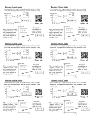
  • 1. Constant  Velocity  Model   Constant  Velocity  Model   From  a  position-­‐time  graph,  an  object's  position  can  be  predicted   From  a  position-­‐time  graph,  an  object's  position  can  be  predicted   based  on  its  starting  position,  velocity,  and  time  interval  of  travel   based  on  its  starting  position,  velocity,  and  time  interval  of  travel   Δx Δx v= v= x f − xi Δt x f − xi Δt slope = slope = t f − ti t f − ti x = vt + xi x = vt + xi Buggy Lab Buggy Lab The object's The object's When velocity is constant, a graph of velocity v. time v = vi displacement is equal to the area When velocity is constant, a graph of velocity v. time v = vi displacement is equal to the area will be a horizontal line under the curve will be a horizontal line under the curve and the velocity at any and the velocity at any time will be equal to the Δx = vt time will be equal to the Δx = vt starting velocity starting velocity Constant  Velocity  Model   Constant  Velocity  Model   From  a  position-­‐time  graph,  an  object's  position  can  be  predicted   From  a  position-­‐time  graph,  an  object's  position  can  be  predicted   based  on  its  starting  position,  velocity,  and  time  interval  of  travel   based  on  its  starting  position,  velocity,  and  time  interval  of  travel   Δx Δx v= v= x f − xi Δt x f − xi Δt slope = slope = t f − ti t f − ti x = vt + xi x = vt + xi Buggy Lab Buggy Lab The object's The object's When velocity is constant, a graph of velocity v. time v = vi displacement is equal to the area When velocity is constant, a graph of velocity v. time v = vi displacement is equal to the area will be a horizontal line under the curve will be a horizontal line under the curve and the velocity at any and the velocity at any time will be equal to the Δx = vt time will be equal to the Δx = vt starting velocity starting velocity Constant  Velocity  Model   Constant  Velocity  Model   From  a  position-­‐time  graph,  an  object's  position  can  be  predicted   From  a  position-­‐time  graph,  an  object's  position  can  be  predicted   based  on  its  starting  position,  velocity,  and  time  interval  of  travel   based  on  its  starting  position,  velocity,  and  time  interval  of  travel   Δx Δx v= v= x f − xi Δt x f − xi Δt slope = slope = t f − ti t f − ti x = vt + xi x = vt + xi Buggy Lab Buggy Lab The object's The object's When velocity is constant, a graph of velocity v. time v = vi displacement is equal to the area When velocity is constant, a graph of velocity v. time v = vi displacement is equal to the area will be a horizontal line under the curve will be a horizontal line under the curve and the velocity at any and the velocity at any time will be equal to the Δx = vt time will be equal to the Δx = vt starting velocity starting velocity