InstructionsView CAAE Stormwater video Too Big for Our Ditches.docx

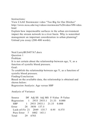
Instructions:
View CAAE Stormwater video "Too Big for Our Ditches"
http://www.ncsu.edu/wq/videos/stormwater%20video/SWvideo.
html
Explain how impermeable surfaces in the urban environment
impact the stream network in a river basin. Why is watershed
management an important consideration in urban planning?
Unload you essay (200-400 words).
Neal.LarryBUS457A7.docx
Question 1
Problem:
It is not certain about the relationship between age, Y, as a
function of systolic blood pressure.
Goal:
To establish the relationship between age Y, as a function of
systolic blood pressure.
Finding/Conclusion:
Based on the available data, the relationship is obtained and
shown below:
Regression Analysis: Age versus SBP
Analysis of Variance
Source DF Adj SS Adj MS F-Value P-Value
Regression 1 2933 2933.1 21.33 0.000
SBP 1 2933 2933.1 21.33 0.000
Error 28 3850 137.5
Lack-of-Fit 21 2849 135.7 0.95 0.575
Pure Error 7 1002 143.1
Total 29 6783

Model Summary
S R-sq R-sq(adj) R-sq(pred)
11.7265 43.24% 41.21% 3.85%
Coefficients
Term Coef SE Coef T-Value P-Value VIF
Constant -18.3 13.9 -1.32 0.198
SBP 0.4454 0.0964 4.62 0.000 1.00
Regression Equation
Age = -18.3 + 0.4454 SBP
It is found that there is an outlier in the dataset, which
significantly affect the regression equation. As a result, the
outlier is removed, and the regression analysis is run again.
Regression Analysis: Age versus SBP
Regression 1 4828.5 4828.47 66.81 0.000
SBP 1 4828.5 4828.47 66.81 0.000
Error 27 1951.4 72.27
Lack-of-Fit 20 949.9 47.49 0.33 0.975
Pure Error 7 1001.5 143.07
Total 28 6779.9
Model Summary

8.50139 71.22% 70.15% 66.89%
Coefficients
Constant -59.9 12.9 -4.63 0.000
SBP 0.7502 0.0918 8.17 0.000 1.00
Regression Equation
Age = -59.9 + 0.7502 SBP
The p-value for the model is 0.000, which implies that the
model is significant in the prediction of Age. The R-square of
the model is 70.2%, implies that 70.2% of variation in age can
be explained by the model
Recommendation:
The regression model Age = -59.9 +0.7502 SBP can be used to
predict the Age, such that over 70% of variation in Age can be
explained by the model.
Question 2
Problem:
It is not sure that whether the factors X1 to X4 which represents
four different success factors have any influences on the annual
savings as a result of CRM implementation.
Goal:
To determine which of the success factors are most significant
in the prediction of a successful CRM program, and develop the
corresponding model for the prediction of CRM savings.
Finding/Conclusion:
shown below:

Regression Analysis: Y versus X1, X2, X3, X4
Regression 4 2667.90 666.975 111.48 0.000
X1 1 25.95 25.951 4.34 0.071
X2 1 2.97 2.972 0.50 0.501
X3 1 0.11 0.109 0.02 0.896
X4 1 0.25 0.247 0.04 0.844
Error 8 47.86 5.983
Total 12 2715.76
Model Summary
2.44601 98.24% 97.36% 95.94%
Coefficients
Constant 62.4 70.1 0.89 0.399
X1 1.551 0.745 2.08 0.071 38.50
X2 0.510 0.724 0.70 0.501 254.42
X3 0.102 0.755 0.14 0.896 46.87
X4 -0.144 0.709 -0.20 0.844 282.51
Regression Equation
Y = 62.4 + 1.551 X1 + 0.510 X2 + 0.102 X3 - 0.144 X4
Correlation: Y, X2, X4
Y X2

X2 0.816
0.001
X4 -0.821 -0.973
0.001 0.000
Based on the analysis of VIF and the correlations, it can be seen
that there is a strong negative correlation between X2 and X4.
Since X4 has a stronger correlation with Y, X2 is discarded and
the regression analysis is run again.
Regression Analysis: Y versus X1, X3, X4
Regression 3 2664.93 888.31 157.27 0.000
X1 1 124.90 124.90 22.11 0.001
X3 1 23.93 23.93 4.24 0.070
X4 1 1176.24 1176.24 208.24 0.000
Error 9 50.84 5.65
Total 12 2715.76
Model Summary
2.37665 98.13% 97.50% 96.52%
Coefficients
Constant 111.68 4.56 24.48 0.000
X1 1.052 0.224 4.70 0.001 3.68
X3 -0.410 0.199 -2.06 0.070 3.46
X4 -0.6428 0.0445 -14.43 0.000 1.18

Regression Equation
Y = 111.68 + 1.052 X1 - 0.410 X3 - 0.6428 X4
The p-value of X3 is greater than 0.05. As a result it is also
discarded. The analysis is run again.
Regression Analysis: Y versus X1, X4
Regression 2 2641.00 1320.50 176.63 0.000
X1 1 809.10 809.10 108.22 0.000
X4 1 1190.92 1190.92 159.30 0.000
Error 10 74.76 7.48
Total 12 2715.76
Model Summary
2.73427 97.25% 96.70% 95.54%
Coefficients
Constant 103.10 2.12 48.54 0.000
X1 1.440 0.138 10.40 0.000 1.06
X4 -0.6140 0.0486 -12.62 0.000 1.06
Regression Equation

Y = 103.10 + 1.440 X1 - 0.6140 X4
Both of the coefficients for X1 and X4 are significantly
different from zero, with p-value being 0.000 for both of the
coefficients. The p-value of overall model is also 0.000, and
thus it is significant in predicting the CRM savings. The R-
square of the model is 97.25%, which implies that 97.25% of
the variation in CRM savings can be explained by the model.
The prediction model is given by: 103.10 + 1.440X1 -0.6140X4
Recommendation:
Since both X1 and X4 are both strongly correlated to the CRM
savings, it is essential to ensure that both X1 and X4 are present
in the implementation of CRM system.
The prediction model obtained can be used in estimating the
CRM savings, given that no other success factors are being
incorporated, and the data used for estimation are within the
ranges of the analysis here.
Question 3
Problem:
It is not sure whether any of the case load, DRG type, case
severity and patient follow-up time are significant in
influencing the high readmission rates, where readmissions are
very expensive and produce tremendous hardship for patients.
Goal:
To determine which of the factors of case load, DRG type, case
severity and patient follow-up time are significant in the
prediction of readmission rates, and develop the corresponding
measure to reduce the readmission rates.
Finding/Conclusion:
shown below:
From the matrix plot, it can be seen that there is a quadratic
relationship between the Readmission rate and the Time. As a
result, a quadratic term of Time will be included in the

regression model.
Regression Analysis: ReadmitRate versus Census, Severity,
Time, DRG
Method
Categorical predictor coding (1, 0)
Regression 6 0.013839 0.002306 63.72 0.000
Census 1 0.000115 0.000115 3.18 0.088
Severity 1 0.000095 0.000095 2.61 0.120
Time 1 0.005527 0.005527 152.69 0.000
DRG 2 0.000032 0.000016 0.44 0.649
Time*Time 1 0.005740 0.005740 158.57 0.000
Error 22 0.000796 0.000036
Total 28 0.014635
Model Summary
0.0060165 94.56% 93.07% 90.34%
Coefficients
Constant -1.0356 0.0840 -12.33 0.000
Census 0.000039 0.000022 1.78 0.088 2.39
Severity -0.001489 0.000921 -1.62 0.120 2.81
Time 0.1661 0.0134 12.36 0.000 526.86
DRG

B 0.00274 0.00294 0.93 0.361 1.57
C 0.00158 0.00297 0.53 0.600 1.41
Time*Time -0.006244 0.000496 -12.59 0.000 522.14
Regression Equation
DRG
A ReadmitRate = -1.0356 + 0.000039 Census -
0.001489 Severity + 0.1661 Time
- 0.006244 Time*Time
B ReadmitRate = -1.0329 + 0.000039 Census -
0.001489 Severity + 0.1661 Time
C ReadmitRate = -1.0341 + 0.000039 Census -
0.001489 Severity + 0.1661 Time
All the coefficients except Time are not significantly different
from zero, with p-values of all the coefficient greater than 0.05.
As a result, all of these variables will be discarded.
Regression Analysis: ReadmitRate versus Time
Regression 2 0.013627 0.006814 175.76 0.000
Time 1 0.011221 0.011221 289.43 0.000
Time*Time 1 0.011825 0.011825 305.03 0.000
Error 26 0.001008 0.000039
Lack-of-Fit 22 0.000975 0.000044 5.37 0.057
Pure Error 4 0.000033 0.000008
Total 28 0.014635

Model Summary
0.0062264 93.11% 92.58% 90.75%
Coefficients
Constant -1.0088 0.0654 -15.43 0.000
Time 0.16763 0.00985 17.01 0.000 264.25
Time*Time -0.006375 0.000365 -17.47 0.000 264.25
Regression Equation
ReadmitRate = -1.0088 + 0.16763 Time - 0.006375 Time*Time
All the regression coefficients in the final model is significantly
different from zero, with p-value of both coefficient of Time
and Time^2 being 0.000. The p-value of the overall model is
also 0.000, which implies that the model is significant in
predicting the readmission rate. The residual plots do not
indicate any significant deviation from the assumption of linear
models. The R-square of the model is 93.11%, which implies
that 93.11% of variation in the readmission rate can be
explained by the model.
Prediction for ReadmitRate
Regression Equation
ReadmitRate = -1.0088 + 0.16763 Time - 0.006375 Time*Time
Variable Setting
Time 13.1

Fit SE Fit 95% CI 95% PI
0.0929927 0.0017406 (0.0894149, 0.0965704) (0.0797035,
0.106282)
The median value for Time is 13.1 days. At this value, the
readmission rate is estimated to be about 9.3%
The range within which we can expect the average patient
readmission rate to fall with 95% confidence is between 8.9%
and 9.6%
The rate within which we can expect an individual patient’s
readmission rate to fall with 95% confidence is between 7.9%
and 10.6%
Recommendation:
The regression model found is Readmission rate = -1.0088 +
0.16763 Time -0.006375 Time2
This model can explain more than 93% of variation in
readmission rate, and simply using patient follow-up time to
predict the readmission rate. It is recommended to use the
model for the range of data within those being used in the
analysis.
Question 4
Problem:
It is not sure whether any of the given predictors can be used to
estimate the gas mileage
Goal:
To determine the best model using the predictor variables that
can estimate the gas mileage.
Finding/Conclusion:
First of all, there are two observations with missing values and
they are being removed.
Based on different trial of combinations of predictors, the final
best model is shown below:
Regression Analysis: Y versus X1

Regression 2 934.00 466.998 61.47 0.000
X1 1 209.46 209.461 27.57 0.000
X1*X1 1 67.77 67.768 8.92 0.006
Error 27 205.11 7.597
Lack-of-Fit 16 142.13 8.883 1.55 0.232
Pure Error 11 62.98 5.725
Total 29 1139.11
Model Summary
2.75621 81.99% 80.66% 77.59%
Coefficients
Constant 39.98 2.56 15.61 0.000
X1 -0.1059 0.0202 -5.25 0.000 20.89
X1*X1 0.000109 0.000036 2.99 0.006 20.89
Regression Equation
Y = 39.98 - 0.1059 X1 + 0.000109 X1*X1
It is found that the best model only used X1 as the predictor
variable. Both X1 and X12 have p-value of 0.000 for the
estimated coefficient. The R-square of the model is 81.99%,
which implies that 81.99% of variation in the gas mileage can
be explained by the model. The best model is given by Gas
mileage = 39.98 – 0.1059X1 + 0.000109 X12.

Recommendation:
The model using only X1 as the predictor variable is
recommended. This is due to its simplicity while at the same
time can explain more than 80% of variation of gas mileage.
220200180160140120100
80
70
60
50
40
30
20
10
S11.7265
R-Sq43.2%
R-Sq(adj)41.2%
SBP
A
g
e
Fitted Line Plot
Age = - 18.35 + 0.4454 SBP
180170160150140130120110
70
60
50
40
30
20
10
S8.50139
R-Sq71.2%
R-Sq(adj)70.2%
SBP

A
g
e
Fitted Line Plot
Age = - 59.86 + 0.7502 SBP
0.10
0.05
0.00
90075060023.021.520.0
900
750
600
10
5
0
23.0
21.5
20.0
0.100.050.00
15.0
12.5
10.0
105015.012.510.0
R
e
a
d
m
i
t
R
a
t
e
C
e

n
s
u
s
S
e
v
e
r
i
t
y
B
M
I
ReadmitRate
T
i
m
e
CensusSeverityBMITime
Matrix Plot of ReadmitRate, Census, ... vs ReadmitRate,
Census, ...
0.010.00-0.01
99
90
50
10
1
Residual
P
e
r
c
e
n

t
0.100.080.060.040.02
0.01
0.00
-0.01
Fitted Value
R
e
s
i
d
u
a
l
0.0150.0100.0050.000-0.005-0.010
8
6
4
2
0
Residual
F
r
e
q
u
e
n
c
y
282624222018161412108642
0.01
0.00
-0.01
Observation Order
R

e
s
i
d
u
a
l
Normal Probability PlotVersus Fits
HistogramVersus Order
Residual Plots for ReadmitRate
Larry Neal
Assignment 6
BUS 457
11/09/2014
Question 1
Problems:
It is not sure whether meeting the daily patient discharge target
is dependent upon the number of consulting MD’s available.
Goals:
To determine whether dependency exists between discharge
target and number of consulting MD’s, and make adjustment for
a balanced approach to staffing for discharge purposes.
Findings / Conclusion:
Chi-square test is being used in the analysis. The result of the
analysis is shown below:
Rows: Met_Discharges Columns: Consulting MDs
0 1 2 3 All
No 95 148 95 54 392
92.75 152.80 91.29 55.16

Yes 95 165 92 59 411
97.25 160.20 95.71 57.84
All 190 313 187 113 803
Cell Contents: Count
Expected count
Pearson Chi-Square = 0.744, DF = 3, P-Value = 0.863
Likelihood Ratio Chi-Square = 0.744, DF = 3, P-Value = 0.863
From the result of the chi-square test, the p-value of the chi-
square test is 0.863. Since the p-value is greater than 0.05, the
null hypothesis cannot be rejected and there is not sufficient
evidence to conclude that dependency exists between discharge
target and number of consulting MD’s
Recommendation:
Other factors instead of number of consulting MD’s should be
investigated to improve meeting patient discharge targets.
Question 2a
Problems:
It is not sure whether annual sales volume is dependent upon
sales proposal being won or lost over 2 years period.
Goals:
To determine whether dependency exists between annual sales
volume and sales proposal being won or lost.
Rows: Proposal Columns: Sales$
<1M >5M 1-2M 2-5M All

Lost 25 30 31 41 127
20.95 29.21 29.21 47.63
Won 8 16 15 34 73
12.05 16.79 16.79 27.38
All 33 46 46 75 200
Expected count
From the result of the chi-square test, the p-value of the chi-
square test is 0.170. Since the p-value is greater than 0.05, the
null hypothesis cannot be rejected and there is not sufficient
evidence to conclude that dependency exists between annual
sales volume and sales proposal being won or lost.
Recommendation:
Other factors instead of sales volume or in addition to volume
should be investigated to identify factors that can increase the
number of sales proposals won.
Question 2b
Problems:
It is not sure whether annual sales volume conditional on
seniority and company car is dependent upon sales proposal
being won or lost over 2 years period.
Goals:
To determine whether dependency exists between annual sales
volume and sales proposal being won or lost, conditional on
seniority and company car.

analysis conditional on seniority is shown below:
Tabulated Statistics: Proposal, Sales$, Seniority
Results for Seniority = <5years
<1M >5M 1-2M 2-5M All
Lost 13 11 16 22 62
8.857 13.918 13.918 25.306
1.9378 0.6119 0.3113 0.4319
Won 1 11 6 18 36
5.143 8.082 8.082 14.694
3.3373 1.0539 0.5362 0.7439
All 14 22 22 40 98
Expected count
Contribution to Chi-square
Results for Seniority = 5+years
<1M >5M 1-2M 2-5M All

Lost 12 19 15 19 65
12.11 15.29 15.29 22.30
0.00096 0.89796 0.00566 0.48942
Won 7 5 9 16 37
6.89 8.71 8.71 12.70
0.00169 1.57750 0.00994 0.85978
All 19 24 24 35 102
Expected count
From the result of the chi-square test conditional on the layer of
seniority, it can be seen that for the layer with seniority less
than or equal to 5 years, the p-value of the chi-square test is
0.030. Since the p-value is smaller than 0.05, the null
hypothesis is rejected and there is sufficient evidence to
conclude that dependency exists between annual sales volume
and sales proposal being won or lost for those with seniority
less than or equal to 5 years.
The result of the analysis conditional on seniority is shown
below:
Tabulated Statistics: Proposal, Sales$, CompanyCar
Results for CompanyCar = No
<1M >5M 1-2M 2-5M All

Lost 12 17 11 24 64
9.06 16.91 11.47 26.57
0.95660 0.00053 0.01940 0.24786
Won 3 11 8 20 42
5.94 11.09 7.53 17.43
1.45768 0.00080 0.02956 0.37769
All 15 28 19 44 106
Expected count
Results for CompanyCar = Yes
<1M >5M 1-2M 2-5M All
Lost 13 13 20 17 63
12.06 12.06 18.10 20.78
0.0726 0.0726 0.2004 0.6865
Won 5 5 7 14 31
5.94 5.94 8.90 10.22
0.1476 0.1476 0.4072 1.3951
All 18 18 27 31 94

Expected count
From the result of the Chi-square test, it can be seen that the p-
values for not having company car and having company car are
0.378 and 0.372 respectively. Therefore it can be conclude that
regardless of having company car, the sales volume and
proposal win or loss numbers are not significantly dependent.
Recommendations:
Lower seniority salespersons are more adept at winning the
proposals with less than one million dollars than higher
seniority salespersons. Therefore low seniority staff should be
assigned to lower payoff clients initially. Company car will not
be a valid motivation factor in sales and thus should not be
used.
Question 3a
Problems:
It is not sure whether authorization errors for medical services
are dependent upon department.
Goals:
To determine whether dependency exists between authorization
errors for medical services and department.
Rows: defect Columns: dep cd
DEP EE SP All

No 16 55 12 83
17.15 52.57 13.28
0.0775 0.1126 0.1234
Yes 15 40 12 67
13.85 42.43 10.72
0.0961 0.1395 0.1528
All 31 95 24 150
Expected count
value is 0.704. Since the p-value is greater than 0.05, the null
hypothesis cannot be rejected. Therefore there is not sufficient
evidence to conclude that dependency exists between
authorization errors for medical services and department.
Recommendations:
Department is not a significant factor in influencing
authorization errors, and thus other factors should be explored.
Question 3b
Problems:
It is not sure whether authorization errors for medical services
are dependent upon case entry site.
Goals:
To determine whether dependency exists between authorization
errors for medical services and case entry site.
Rows: defect Columns: Case Enter Site

HOU PDX PHL SD SFO All
No 11 17 26 7 22 83
10.51 18.26 26.56 6.09 21.58
0.02253 0.08694 0.01181 0.13705 0.00817
Yes 8 16 22 4 17 67
8.49 14.74 21.44 4.91 17.42
0.02791 0.10771 0.01463 0.16978 0.01013
All 19 33 48 11 39 150
Expected count
* NOTE * 1 cells with expected counts less than 5
value is 0.963. Since the p-value is greater than 0.05, the null
hypothesis cannot be rejected. Therefore there is not sufficient
evidence to conclude that dependency exists between
authorization errors for medical services and case entry site.
Recommendations:
Case entry site is not a significant factors in influencing
authorization errors, and thus other factors should be explored.
However, it should be noted that the expected cell count for San
Diego (SD) logging a “Yes” response is less than 5, it is
recommended that more data to be collected with the response
for San Diego (SD) logging being “Yes” such that the count of

data is greater than 5. The test is suggested to be redone at that
time.
Larry Neal
Assignment 5
BUS 457
10/31/2014
Q1.
Problem:
For a supply chain project team it is not certain whether
international orders placed on weekends is longer than that of
those placed on a weekday, which is 3 days. The team will
pursue weekend shipment time improvements only if it is
proven that the median weekend order shipments are
significantly longer than 4 days.
Goal:
Determine whether the median weekend order shipments are
significantly longer than 4 days.
Findings / Conclusions:
A Wilcoxon signed rank test is carried out to test for the
median. The result is shown below:
Wilcoxon Signed Rank Test: ShipTime
Test of median = 4.000 versus median > 4.000
N for Wilcoxon Estimated
N Test Statistic P Median
ShipTime 37 30 351.0 0.008 6.500
From the result, it can be seen that the p-value of the test is
0.008. Therefore the null hypothesis is rejected at 5%
significant level. There is sufficient statistical evidence to infer
the median ship time for weekend international order is
significantly longer than 4.0 days.

Recommendation:
Pursue weekend international orders improvements as a means,
in part, to bring weekend shipments more in line with the week
day shipment median of 3.0 days.
Q2
Problem:
Verify the theory that the patient length of stay is generally
longer when they miss the target of patient discharge than when
they don’t.
Goal:
Determine whether the length of stay is longer when they miss
the patient discharge target than when they don’t.
A Mann-Whitney test is carried out to test for the hypothesis of
median length of stay whether missing the patient discharge
target is longer than when not. The result of the test is shown
below:
Mann-Whitney Test and CI: LOS_No, LOS_Yes
N Median
LOS_No 392 2.0000
LOS_Yes 411 2.0000
Point estimate for η1 - η2 is -0.0000
95.0 Percent CI for η1 - η2 is (-0.0001,0.0001)
W = 158801.0
Test of η1 = η2 vs η1 > η2 is significant at 0.3556
The test is significant at 0.3523 (adjusted for ties)
Based on the result of the test, the p-value is 0.3523. Therefore
the null hypothesis is not rejected. There is not sufficient
evidence to conclude that the median length of stay when they
miss the target is longer than when they don’t.

Recommendation:
Whether meeting the patient discharge targets has no influence
on the patient length of stay, and thus other factors should be
considered when it is intended to adjust for length of stay.
Q3
Problem:
It is uncertain that which of the factors among hospitalist group,
number of consulting MDs and payer have significant influence
on the excessive patient length of stay at Basin Medical Center.
Goal:
Determine which, if any of the factors of hospitalist group,
number of consulting MDs and payer have significant influence
on excessive patient length of stay.
Since the research data are subject to outliers and are not
normally distributed, Mood’s Median nonparametric test was
used to carry out the hypothesis test. The result of test between
length of stay and hospitalist groups is shown below:
Mood Median Test: LOS versus Hospitalist Group
Mood median test for LOS
Chi-Square = 4.30 DF = 2 P = 0.116
Hospitalist Individual 95.0% CIs
Group N≤ N> Median Q3-Q1 ---+---------+---------+----
-----+---
Galen 129 150 3.00 3.00 (--------------------------------*
n/a 243 211 2.00 1.00 *--------------------------------)
Pediatrix 39 31 2.00 1.00 *--------------------------------)
---+---------+---------+---------+---
2.10 2.40 2.70 3.00
Overall median = 2.00
Based on the result of the test, it is found that the p-value of the
test is 0.116. Therefore the null hypothesis is not rejected, and

there are not sufficient evidence to conclude that median length
of stay is different among hospitalist groups.
The result of the test between the length of stay and number of
consulting MDs is shown below:
Mood Median Test: LOS versus Number of Consulting MDs
Chi-Square = 88.39 DF = 3 P = 0.000
Number of
Consulting Individual 95.0% CIs
MDs N≤ N> Median Q3-Q1 ---+---------+---------+-----
----+---
0 133 57 2.00 1.25 *
1 175 138 2.00 2.00 *
2 85 102 3.00 2.00 (-------*
3 18 95 5.00 6.00 (--------*-------)
---+---------+---------+---------+---
2.4 3.6 4.8 6.0
test is 0.000. Therefore the null hypothesis is rejected, and there
are sufficient evidence to conclude that median length of stay is
different among consulting MDs with three consulting MDs
produced a median length of stay of 5 days.
The result of the test between the length of stay and payer is
shown below:
Mood Median Test: LOS versus Payer
Chi-Square = 51.31 DF = 6 P = 0.000

Payer N≤ N> Median Q3-Q1
Commercial 135 108 2.00 2.00
County 50 36 2.00 1.00
MediCal 76 61 2.00 1.00
Medicare 90 162 3.00 3.00
Other General Ins 18 0 1.00 1.00
Self Pay 33 23 2.00 3.00
Sutter Select 9 2 2.00 1.00
Individual 95.0% CIs
Payer +---------+---------+---------+------
Commercial *---------)
County *---------)
MediCal *---------)
Medicare *---------)
Other General Ins *---------)
Self Pay *---------)
Sutter Select (---------*)
+---------+---------+---------+------
1.0 2.0 3.0 4.0
test is 0.000. Therefore the null hypothesis is rejected, and there
are sufficient evidence to conclude that median length of stay is
different among payer type with payer type of Medicare
produced a median length of stay of 3 days.
Recommendations:
In order to solve the problem of excessive length of stay, the
number of consulting MDs should be limited to two at most, and
means in reducing excessive length of stay should focus on
those who receive Medicre benefits.

4.
Problem:
It is interested to know whether different types of Enterprise
Resource Planning software influence the purchasing decision
for the customer, and a survey is carried out to ask for the
customers’ opinion on it.
Goal:
Determine whether features in ERP software has influence on
customer purchase decisions. If so, identify which type of ERP
software is most influential.
Since the data are not subject to outliers and the data are not
normally distributed, a Kruskal-Wallis nonparametric test is
selected for the research analysis.
The result of the test is shown below:
Kruskal-Wallis Test: Response versus ERPtype
Kruskal-Wallis Test on Response
ERPtype N Median Ave Rank Z
A 1 3.000 9.5 -0.25
B 8 2.500 8.2 -1.63
C 2 2.000 5.0 -1.44
D 9 8.000 15.7 2.98
E 1 2.000 5.0 -0.99
Overall 21 11.0
H = 9.60 DF = 4 P = 0.048
H = 10.03 DF = 4 P = 0.040 (adjusted for ties)
* NOTE * One or more small samples
Based on the result of the test, the p-value is 0.040. The null
hypothesis is rejected at 5% significant level. There is sufficient
evidence to conclude that there is significant differences in
median response on the survey question of the opinion on

whether the ERP software features influence the purchase
decision. From the median, it can be seen that ERP type D has
the largest median response to this question.
Recommendation:
Since the ERP type D has the largest satisfaction, the marketing
strategy should be on promoting the feature of ERP type D
software. More resources should be placed in further
development on the features of ERP type D, and less resources
should be put on other ERP types of software.
Question 1
1. When considering analysis of research data, which is a
characteristic we look for?
Spread in the data
Location (central tendency of the data)
Shape of the data
Stability of the data
All of the above
5 points
Question 2
1. Which of the following describes the data observation that
occurs most frequently?

Mean
Median
Mode
Range
Standard deviation
5 points
Question 3
1. What is σ (sigma) a measure of?
Location
Spread
Stability
Mean
Mode
5 points
Question 4
1. Which test is best to test the hypothesis that multiple
variances (2 or more) are equal?

t test
proportions test
Mood's median test
Levene's test
Analysis of Variance (ANOVA)
5 points
Question 5
1. In the sampling, hypothesis testing and analysis of business
research data, which of the following is true?
We make inferences about the population parameters based on
sample statistics
The sample should be representative of the population
A larger sample size is always better
Answers1 and 2 only
Answers 1, 2 and 3
5 points
Question 6

1. What is the advantage of a dot plot over a histogram?
Preserves the original data in the plot
Shows shape of the data in the plot
Shows spread of the data in the plot
Shows central location of the data
Shows priority of categories
5 points
Question 7
1. What is the name of the research data analysis tool shown
below?
Histogram
Pareto chart
Bar graph
Box plot
Line plot

5 points
Question 8
1. What is the implication of a data distribution with mean,
median and mode being approximately equal?
The spread in the data are equal
The data are unstable
The data can not be plotted using a Histogram
The data are normally distributed
The data can not be plotted using a Box Plot
5 points
Question 9
1. Which test is best to assess whether two independent means
are equal?
2-sample t test
Levene's test
paired t test
one proportion test

two proportions test
5 points
Question 10
1. Which test is best to assess whether the % defective is the
same between two independent business units?
2 sample t test
Levene's test
paired t test
one proportion test
two proportion test
5 points
Question 11
1. A researcher’s hypothesis to test for equality of means at
95% confidence was rejected with a p-value of 0.01. What is
the chance the researcher is wrong about this 'reject' decision?
95%
5%
1%

99%
impossible to tell without further analysis
5 points
Question 12
1. A researcher’s hypothesis to test for equality of means (i.e., 2
sample t test) at 95% confidence was accepted with a p-value of
0.25 What is the chance the researcher is wrong about this
"accept" decision?
95%
5%
25%
75%
impossible to tell without further analysis
5 points
Question 13
1. Refer to the Minitab output below. The results of a statistical
test at 95% confidence (significance level of 0.05) to determine
the difference in the average amount of time to process a legible
insurance claim vs. an illegible insurance claim are below.
What is the decision?

continue to process legible insurance claims
accept the null hypothesis
reject the null hypothesis
continue to process both legible and illegible insurance claims
the amount of time to complete a legible claim is about the
same as an illegible claim
5 points
Question 14
1. Refer to the Minitab output below. What is the research
hypothesis under consideration?
Ho: σ21 = σ22
Ho: π1 = π2
Ho: µ21 = µ22
Ho: µ1 = µ2
Ho: σ1 = σ2

5 points
Question 15
1. What is the most appropriate research hypothesis for the
following scenario? “Historically, the mortality rate for
particular type of brain surgery is 10%. A new, simpler
technique has been developed that may reduce the mortality
rate?
Ho: σ2 ≤ 10%
Ho: π ≤ 10%
Ho: µ ≤ 10%
Ho: µ1 ≤ µ2
Ho: π1 ≤ π2
5 points
Question 16
1. In managing the risks associated with statistically based
research decisions, which is NOT likely something the
researcher can select?
alpha
beta
delta

sample size
sigma
5 points
Question 17
1. Which is best defined as “the critical difference a researcher
wants to be able to detect”?
alpha
beta
delta
sample size
sigma
5 points
Question 18
1. What is ANOVA?
a stellar event
a PBS program

a type of chevrolet
a statistical research tool to test the hypothesis concerning
equality of multiple variances
a statistical research tool to test the hypothesis
concerming equality of multiple means
5 points
Question 19
1. Refer to the ANOVA output below. A business researcher is
investigating the process inputs that influence late orders
(measured as % late). Which statement is FALSE?
Three factors are being researched simultaneously
There is a chance of a beta error in this analysis
Four different product types were considered in this research
Particular combinations (interactions) of Order Frequency and
Quantity significantly influences late orders
The Order Frequency significantly influences whether an order
is late
5 points

Question 20
1. Refer to the factor plot below. The factor plot shows the
mean percent of time (i.e., 0.15 = 15%) orders are late based on
particular combinations of order quantities and order
frequencies. Which would be a reasonable recommendation
based on this plot?
Look elsewhere (i.e., another factor) to address Late Orders
Address order Quantities between 1 and 3 to help reduce Late
Orders
Address order Quantities greater than 3 to help reduce Late
Orders
Address order Quantities between 1 and 3 where the orders
occur Daily, to help reduce Late Orders
Address order Quantities greater than 3 where the orders occur
Daily, to help reduce Late Orders
Instructions:

Explain the human and natural influences that contributed to the
creation of the Dust Bowl (200-400 words). Upload your work
in MS Word or PDF.
Answer the following questions. Omit Question #19

InstructionsView CAAE Stormwater video Too Big for Our Ditches.docx

Recommended

Recommended

More Related Content

Similar to InstructionsView CAAE Stormwater video Too Big for Our Ditches.docx

Similar to InstructionsView CAAE Stormwater video Too Big for Our Ditches.docx (20)

More from dirkrplav

More from dirkrplav (20)

Recently uploaded

Recently uploaded (20)

InstructionsView CAAE Stormwater video Too Big for Our Ditches.docx