SlideShare uma empresa Scribd logo
1 de 32
Baixar para ler offline
J O U R N A L OF FINANCIAL A N D QUANTITATIVE ANALYSIS      Vol. 44, No. 4, A u g . 2009, p p . 7 4 5 - 7 7 5
COPYRIGHT 2009, MICHAEL G. FOSTER SCHOOL OF BUSINESS, UNIVEHSITY OF WASHINGTON, SEAHLE. WA 98195
doi:1Q.1017/S002210900999010X


Does Prior Performance Affect a Mutual Fund's
Choice of Risk? Theory and Further Empirical
Evidence
Hsiu-lang Chen and George G. Pennacchi*


Abstract
Recent empirical studies of mutual fund competition examine the relation between a fund's
performance, the fund manager's compensation, and ihe finid manager's choice of portfo-
lio risk. This paper models a manager's portfolio choice for compensation rules that can
be either a concave, linear, or convex function of the fund's performance relative to that
of a benchmark. For particular compensation structures, a manager increases the fund's
"tracking error" volatility as its relative perfomiance declines. However, declining perfor-
mance does not necessarily lead the manager to raise the volatility of the fund's return. The
paper presents nonparameiric and parametric tests of the relation between mulua! fund per-
formance and risk taking for more than 6.üt)ü equity mutual funds over the l%2 to 2006
period. There is a tendency for mutual funds to increase the standard deviation of tracking
errors, but not the standard deviation of returns, as their perfomiance declines. This risk-
shifting behavior appears more common for funds whose managers have longer tenures.


I.    Introduction
      As mtitual fund investing has grown, the management of mutual funds has
come under closer scrutiny by financial ecotwmists. One strand of research ex-
amines potential agency problems between a mutual fund's shareholders and its
portfolio manager. Several studies investigate whether a manager might unneces-
sarily shift the fund's risk in response to changes in its performance relative to
other funds. This behavior is linked to the way the manager is compensated and
to the actions of mutual fund investors. The manager's compensation depends on
her success in generating flows of new investments into the fund, while mutual
fund investors "chase returns" by channeling investments into funds with better


    'Chen, hsiulang@uic.edu. College of Business Administration. University of Illinois at Chicago.
601 S. Morgan St.. Chicago. IL 60607; Pennacchi, gpennaccCa'illinois.edu, College of Business. Uni-
versity of Illinois at Urbana-Champaign. 515 E. Gregory Dr.. Champaign, IL 61820. We are grateful
for valuable comments pmvided by Wayne Fersnn (associate editor and referee), Zoran Ivkovich.
Jason Karceski, Maiii Keloharju, Paul Malafesta (Ihe editor), and participants al the 2000 .WA
Meetings and at seminars al llie Federal Reserve Bank of Cleveland, the University of Illinois, the
University of North Carolina at Chapel Hill, and the University of Notre Dame.
                                                    745
746      Journal of Financial and Quantitative Analysis

 relative performance. This creates a situation described as a mutual fund "tour-
 nament," where portfolio managers compete for better performance, greater fund
 inflows, and, ultimately, higher compensation.
       Inflows rise nonlinearly with a fund's relative performance. Numerous stud-
 ies document that mutual funds with the best recent performance experience the
 lion's share of new inflows, but poorly pertbrming funds are not penalized with
sharply higher outflows.' If the fund manager's compensation rises in propor-
tion to the fund's inflows, this convex pertbrmance-fund flow relation produces
a convex performance-compensation structure.^ Research such as Sirri and
Tufano (1998) notes that such compensation is similar to a call option, creat-
ing an incentive for a manager to raise the risk of the fund's relative returns.
Chevalier and Ellison (1997), Brown, Harlow, and Starks (BHS) (1996), Basse
(2001 ), and Goriaev, Nijman, and Werker (GNW) (2005) have empirically exam-
ined the behavior of a cross-section of mutual funds for which this risk-taking
incentive is predicted tti differ.
       The current paper adds to this mutual fund tournament literature by pro-
viding new theoretical and empirical insights into risk taking by mutual funds. It
models the optimal intertemporal portfolio strategy of a mutual fund manager that
faces the competitive tournament environment assumed by recent empirical work.
Explicit solutions for this manager's portfolio allocation are derived when her util-
ity displays constant relative risk aversion and compensation is either a concave,
linear, or convex function of the fund's relative calendar-year performance.
       The model shows that the deviation of a fund manager's optimal portfo-
lio from the benchmark portfolio is a function of the fund's performance. If the
penalty for poor performance is limited so that the manager's total compensation
can never fall to zero, then the fund manager chooses to deviate more from the
benchmark portfolio as the fund's relative performance declines. In other words,
when a fund is performing poorly it displays more "tracking error" than when it
performs relatively well. However, it is not necessarily true that an underperiorm-
ing fund chooses to raise the volatility (standard deviation) of its returns.
       Almost all empirical studies that have tested for tournament risk shifting
have analyzed fund risk measures other than tracking error. Most commonly, em-
pirical research has tested for whether underpertbrming funds increase the stan-
dard deviation of their total returns, rather than the standard deviation of their
tracking errors. The most comprehensive of these studies conclude that there is
no evidence for tournament behavior. However, based on our model's insights.


      'Siudies examining the fund flow-performance relalionship include IppoliUi (1992). Gruber
(1996), Chevalier and Ellison (1997), Sirri and Tufano (1998). Gœtzmann and Peles (1997), and
Del Guercio and Tkac (2002).
     -The literature on mutual fund tournaments distinguishes between a fund's investment advisor,
the entity responsible for ponfoho management, and the portfolio manager hired by the advisor. The
typical investment advisor is paid a fixed fraction of the fund's assets, assets that depend on both net
fund inflows(externali;rowthof assets) and the fund's return (internal growthof assets). However, the
ptirtfoUu manager's compensation is assumed to depend only on his ability lo generate extraordinary
growth in fund assets, growth that depends on the fund's return relative to (the average of) other funds'
rettims. Common or systematic shocks to all funds' returns (affecting internal asset growth) are not
due to the individual manager's ponfolio selection ability and would not alïect compensation. Hence,
compensation is assumed to depend on relative, not absolute, performance.
Chen and Pennacchi       747

we argue that this conclusion may be unwarranted because it is based on tests that
have employed risk measures that are inappropriate for examining the tournament
hypothesis.
      This paper reexamines the empirical evidence for tournament behavior in
light of our model's predictions. We construct two different types of tests. One is
a nonparametric test that modifies the standard deviation ratio (SDR) tests used
in prior studies. It analyzes risk shifting for a cross-section of mutual funds based
on the SDR of their tracking errors, rather than the SDR of their returns. Another
parametric test exatiiines individual mutual funds' time-series behavior based on
an empirical model that nests our paper's theoretical one. Unlike the nonparamet-
ric tests that allow a fund's risk to change only once per year, this parametric test
permits each fund's risk to vary at every (monthly) observation date.
      Both tests are performed using data on tiiore than 6.00() mutual funds that
operated during the 1962 to 2006 period. As predicted by our model, the empirical
evidence suggests that an underpertorming mutual fund manager increases the
standard deviation of tracking error, but not the standard deviation of returns.
Evidence is strongest for managers that have longer tenures at their funds, a result
that also is consistent with our model.
      The plan of the paper is as follows. Section II briefly discusses related the-
oretical and empirical work on the risk-taking incentives of mutual fund man-
agers. In Section III we present our model. Section IV discusses nonparametric
and parametric empirical methods for testing the risk-taking behavior implied by
our model. Section V describes our data, and Section VI presents the empirical
results. Concluding comments are in Section VII.


II.   Related Literature
     This section begins by discussing sotne of the theoretical research that
relates to our paper's model. It then reviews empirical studies of mutual fund
tournaments.

A.    Models of Portfolio Management
      A growing literature examines links between a fund manager's compensa-
tion contract and his portfolio choice. Grinblatt and Titman (1989) show how
compensation contracts that include a bonus for good performance can produce
moral hazard incentives. Mutual fund managers can maximize the present value
of their option-like bonus by choosing a fund portfolio with excessive risk. More-
over, the fund manager can risklessly capture the increased value of this bonus if
she can hedge using her personal wealth.
      Starks (1987) considers the moral hazard incentives of a bonus contract, fo-
cusing on situations of asymmetric information between investors and fund man-
agers. When investors cannot observe a manager's choice of portfolio risk or the
manager's effort level, compensation contracts with symmetric payoffs dominate
contracts that include a bonus. However, Das and Sundaram (2002) show that the
relative advantages of symmetric and bonus contracts can be reversed if investors'
choice of funds is made endogenous to the funds' risk levels and compensation
'r


748    Journal of Financial anä Quantitative Analysis

 contracts. In their model, bonus contracts provide better risk sharing between in-
 vestors and fund managers when investors take account of a fund's risk and con-
tract choice. Dybvig. Farnsworth. and Carpenter (2009) also find that contracts
 should include a bonus proportional to the fund's return in excess of a benchmark
return when a fund manager's effort determines the quality of her information.-'
      Other research, such as Huberman and Kandel ( 1993), Heinkel and Stoughton
 (1994). and Huddart (1999), considers environments where fund managers pos-
 sess different abilities that are unknown to investors. In these screening mod-
els, there is typically an initial period when investors learn of managers* abilities
based on their relative performances, followed by a second period when investors
can switch their savings to those managers perceived to have the highest abilities.
Hence, these "investor learning" models can explain the link between fund flows
and prior performance. In addition, if managerial ability displays decreasing re-
turns to scale. Berk and Green (2004) show that fund flows determine the relative
 sizes of mutual funds such that, in equilibrium, investors expect no future superior
returns net of fund fees and expenses.
      The model in the current paper differs from this previous work by focusing
on how prior performance affects a fund manager's intertemporal choice of port-
folio risk. We take the structure of compensation as given and study a manager's
dynamic portfolio choice during an annual mutual fund tournament. Models by
Carpenter (200Í)), Cuoco and Kaniel (2001), and Basak, Pavlova, and Shapiro
(2007) are related to ours. These papers assume that the performance-related coni-
f>onents of a manager's compensation are piece-wise linear functions of perfor-
mance. Carpenter (2000) specifies compensation equal to a fixed fee plus a call
option written on the value of the managed portfolio with an exercise price equal
to a benchmark asset. Cuoco and Kaniel (2001) permit compensation to contain
a penalty for poor performance in the form of the manager's writing a put option
on the managed portfolio. Basak, Pavlova, and Shapiro (2007) assume a man-
ager's compensation is linear in portfolio returns relative to a benchmark but sub-
ject to fixed minimum and maximum payoffs, equivalent to a bull spread option
strategy.
      While we also assume that a manager's compensation depends on the port-
folio's performance relative to a benchmark, the contract is not strictly in the form
of standard call or put options. Rather than being an option-like, piece-wise lin-
ear function of performance, our compensation contract is a smooth function that
can be concave, linear, or convex in relative performance. An advantage of our
smooth compensation schedule is that it leads to simple and intuitive closed-form
solufions for a fund manager's optimal portfolio choice. This simplicity allows
the model to guide our later empirical tests of mutual fund behavior.
      Arguably, a smooth performance-compensation function better captures the
environment of a mutual fund tournament where compensation is proportional to
a fund's assets under management that, in tum, depend on how investor inflows


    ^Becker, Ferson. Myers, and Schill (1999) also analyze the consequences for portfolio choice
when a manager has compensation based on the fund's return in excess of a benchmark and also has
the ability to time the market.
Chen and Pennacchi             749

respond to the fund's relative performance.'' Chevalier and Ellison (( 1997). p. 1181 )
contend that assuming a smooth relationship between miitu;il fund performance
and fund flows is preferable because it avoids imposing the strong restrictions on
risk incentives that occur with a piece-wise linear contract. Under a piece-wise
linear contract, a manager's risk incentives are always maximized or minimized
at the contract's kink points, yet for mutual funds, identifying the location of these
kink points is subject to error since they must be estimated from past fund flows.

B.   Empirical Research on Mutual Fund Tournaments

      Several empirical studies have analyzed the relationship between a mutual
fund's prior pertbrmance and its choice of risk. Chevalier and Ellison ( 1997) esti-
mate the shape of mutual funds" performance-fund How relation and use it to infer
different funds' risk-taking incentives. They, like other researchers, assume that
a fund's inflows respond primarily to its relative performance calculated over the
previous calendar year. Thus fund managers compete in annual tournaments that
begin in January and end in December.-^ A fund's risk-taking incentive over the
final quarter of the year is assumed to be proportional to the estimated convexity
of fund inflows measured locally around the fund's September performance rank-
ing. Using 1983 to 1993 data on the equity holdings of mutual funds at the ends
of September and December. Chevalier and Ellison (1997) find that a fund tends
to change the standard deviation of its return relative to a benchmark return as the
performance-fund flow relation predicts. For example, young mutual funds that
perform relatively poorly from January to September tend to raise the standard
deviation of their return in excess of a benchmark return (standard deviation of
tracking error) during October to December/'
      Another study by BHS (1996) performs SDR tests of whether a fund that
performs relatively poorly at midyeai- tends to raise the standard deviation of its
return over the latter half of the year more than does a fund that performs relatively
well at midyear. They use monthly returns data for a cross-section of mutual funds
during 1980 to 1991 and ñnd support for the tournament hypothesis that midyear
"losers" gamble to improve their relative end-of-year performance by raising tbeir
funds' standard deviation of returns more than do midyear "winners." Koski and
Pontiff (1999) also use monthly returns data over the 1992 to 1994 period to


    "•The ciinlract in Carpenter {2()(K)} may better represeiU ihe irompensalion of a nonfiniinciiil timi
manager who receives stock options. Cuoco ¡md Kaniel's {2(K)I ) compensation contract miyht be mosl
appropriate for other poritblio managers, such as managers of pension funds. Their analysis focuses
on tlie equilihriuni asset pricing consequences of portfolio management. Basak el ai. (2007) assume a
complete markets environment where portfolio managers lack asset selection ability and choose only
systematic risk.
     ^This assumption is justified because sources of mutual fund information, such as Momingstar,
Inc., typically compute relative fund performances using this calendar-year period. Hence, flows of
investor funds and. in turn, managerial compensation should be most sensitive to a fund's calendar-
year performance- Empirical evidence in Koski and Pontiff ( 1999) indicates that changes in a fund's
risk are most strongly related to performance calculated over calendar years.
     ''Chevalier and Ellison (1997) also test their estimated performance-flow relation using monthly
data on fund returns. They measure a fund's risk as ihe standard deviation of its return in excess of
the return on a value-weighted index of NYSE. AMEX. and NASDAQ stocks and lind thai it moves
in the predicted direclion during ihe last quarter of the year.
750    Journal of Financial and Quantitative Analysis

calculate various measures of a fund's risk, including the standard deviation, beta,
and idiosyncratic risk of a fund's returns. Their results are similar to those of BHS
(1996) in that a mutual fund's performance in the first half of the calendar year is
negatively related to its change in risk during the second half.
      However, more recent research finds that some of these results are not ro-
bust to other testing methods and sample periods. Busse {2001) uses a different
database of daily, rather than monthly, mutual fund returns from 1985 to 1995
to calculate more accurate estimates of a fund's SDRs. He duplicates the SDR
tests in BHS (1996) and finds no evidence that midyear poor-performing funds
increase their standard deviation of return more than midyear better-performing
funds. He also shows that if standard deviations are calculated using monthly re-
turns measured from the middle of each month, rather than from the beginning of
each month as in BHS ( 19%), the evidence disappears for raising return standard
deviations as relative performance declines.
      Similariy. GNW (2005) replicate BHS's (19%) SDR tests using an expanded
 1976 to 2001 sample of monthly fund returns and correct their test significance
levels for cross-correlation in fund returns. They also find no evidence that un-
derperfonning funds raise their standard deviations of returns. Hence, the more
comprehensive studies of Busse (2001 ) and GNW (2005) conclude that the BHS
(1996) finding of tournament behavior is fragile. It does not hold up to more pre-
cise tests and larger samples of mutual fund returns.
      As our model of mutual fund tournaments in the next section demonstrates,
under plausible conditions, an optimizing manager chooses to raise the standard
deviation of her fund's tracking error (return in excess of a benchmark) as the
fund's relative performance declines. Such behavior does not necessarily imply
a rise in the fund's standard deviation of returns, beta, or residual risk. Hence,
with the exception of Chevalier and Ellison (1997). prior tests of tournament be-
havior are based on arguably inappropriate risk measures. In particular. Busse's
(2001) and GNW's (2005) rejection of tournament behavior may be unjustified
since their SDR tests, like those of BHS (1996). employ standard deviations of
total returns, rather than tracking error. Reexamining the evidence for tournament
behavior with a focus on mutual funds' tracking errors, rather than their total
returns, motivates our paper's empirical work.


III.   Modeling a Mutual Fund Manager's Portfolio Decisions
      We now describe our model's specific assumptions. A fund manager's com-
pensation is assumed to depend on tbe fund's performance relative to a benchmark
index. The fund's portfolio can be invested partly in this benchmark index and
partly in a set of "alternative" securities cbosen by its fund manager. These alter-
native securities are defined as the portion of the fund's total assets that accounts
for the difference between the fund's portfolio and one that is invested solely in
the benchmiu-k portfolio. Tbe Appendix shows that when securities' excess re-
turns and return covariances are conslant, the fund manager's optimal choice of
individual alternative securities is one where their relative portfolio proportions
do not vary over time. This implies that tbe manager's intertemporal portfolio
choice problem can be transformed to one of allocating a portion of the fund's
Chen and Pennacchi            751

portfoiio to tiie i^enchmarii index and the remaining portion to a single alternative
composite security.' Hence, we simplify the presentation by assuming at the start
that the portfoiio allocation prohiem involves only two types of securities: the
benchmark index and a single alternative security.
      Defme 5, as the value of the relevant benchmark index at date / and A, as the
date / value of the alternative securities. Then 5, and A, are assumed to follow the
processes

                                   àS                     .       .      .
(I)                                —      =     asdt + asdz            and

(2)                                —     =     aAdt + aAdq>

where tT^rf-fT.Aí/^—tTAsííí-For analytical convenience,CT^.0-5. and (Tasare assumed
to be constants. Here, a^ and as may be time varying, as might be the case if
market interest rates are stochastic.** However, we require that the spread between
their expected rates of return, o^ - as. be constant.
      If the fund manager allocates a portfolio proportion of 1 -u; to the benchmark
index and a proportion ui to the alternative securities, then the portfolio's value,
V. follows the process

                 dV           ,,        JS        dA
(3)              y      -     (l-.^)y.^^
                        =     [( 1 — u;) Qs + U;Û;^] dt + (]      — uj) fT


Note that whenever CJ ^ 0, the fund's return in equation (3) deviates from the
benchmark return. We can also calculate the process followed by the fund's rela-
tive performance. Define G, = V¡/S, to be the date t ratio of the value of a share of
the fund's portfolio to that of the benchmark. A simple application of Itô's lemma
shows that

(4)              —r      =    uj(aA-      as + o-¡ - ffAs) ät + uj [aAdq - asdz).
                  Lf

     The fund manager is assumed to compete in a tournament for inflows into
the fund. At the start of the tournament's assessment period. G = 1 by definition,
but it then changes stochastically according to equation (4). Thus, G, measures
the date t ratio of the fund's return to that of the benchmark since the start of the
tournament, and hence D, ^ ln(G,) is the difference between the fund's contin-
uously compounded return and that of the benchmark index since the beginning
of the tournament.^ The tournament ends at date 7", which, for example, could be


     'This "two-fund separaiion" resull is similar to Merton's ( 1971 ) case of lognormal asset prices.
     ^The Appendix derives the values of a, and a^ in terms of the p:irameters o!" processes for n
individual altemalive securities.
     ^We refer to relative performance as the ratio of returns. G,. rather than the difference in returns.
Dr. but this distinction is nonessential. The manager's compensation function could be rewritten in
terms of In (Gf). rather than G,. As will be shown, a manager's optimal portfolio choice is independent
of prior performance when compensation is proportional to a power of G, rather than D,, so the ratio
is a natural variable to use.
752      Journal of Financial and Quantitative Analysis

the last trading day of the calendar year. The manager's compensation is a func-
tion of the fund's relative perfonnance at the end of the tournament, so that his
compensation or "pay" can be written as /'[G7].'"'"
      The fund manager maximizes his expected utility of compensation (wealth)
at the end of the tournament by choosing the fund's asset allocation at each point
in time during the assessment period.'^ This maximization problem can be written
as

(5)                                      Max              E.{U{PIGT])],
                                     uj{.,) V sç[,,T]

subject to the process followed by G given in equation (4). If we define J{G, t)
as the derived utility of wealth (or performance) function, then assuming that
U{P[GT]) is concave in Gj, the first-order condition of the Bellman equation
with respect to u; implies that the portfolio proportion invested in the alternative
securities is

(0)                                     ÜJ     —


where « c = QA - as +CT|- (TAS and (J¿- ^ ffj - 2(T^5 + «rj. Substituting this back
into the Belltnan equation, one obtains an equilibtium partial differential equation
for J that must satisfy the boundary condition J{GT, T) = U(P[GT]). A solution
requires that the manager's utility function and compensation schedule be speci-
fied. We make the standard assumption that utility displays constant relative risk
aversion, U{P[GT]) — {P[GT)'' /-y, where 7 < 1. For the manager's compensation
schedule, we choose a flexible specification that can be either a concave, linear,
or convex function of fund performance:


(7)                                P[GT]         -

where b > 0, c > 0, a > -b/c, and c-y < 1. When 0 < c < I. the manager's
compensation is a concave function of performance. Gr- Compensation is linear


    '"In practice, compensation may depend also on the performance of the ovenill equily (mutual
fund) market. Kareeski (:îOO2) shows thai a fund's inflows are highest when the fund performs rela-
tively well and. simultaneously, the overall stock markei performs well. He studies the implications
of ihis pheTH)menon ¡br fund managers' selection of high versus low beta stocks and the equilibrium
etïecls on as.sei prices. Our analysis omils (his market effect.
    ' The assumption that compensation depends only on ihe fund's performance relallve to a single
index is a simplificaiion for another reasim. In general, a fund's nei inflows, and hence ils manager's
portfolio choices, might depend on the iinal pertonnances of each of the mutual fund's compeiitors.
Oursimplitied siructure can be justified i]i an environment where there arc a large (intiniie) number of
mutual funds that choose dilferenl "altemaiive" securities. Their relative performances over the year
wmild be a smooth, approximately normally distributed function around a mean performance. This
would justify (as we do in our empirical work) using the "average" performance of all mutual funds
as a sufficieni statistic for comparing any given mutual fund's performance.
    '•'Our model selling is very similar lo thai of Diitfie and Richardson (1991), who study ihe trading
strategy of a risk-averse hedger. We assume that the manager does noi hedge his compensation risk
via his personal ponfolio. This is a standard assumption, though Grinblatt and Titman (1989) is an
exceplion.
Chen and Pennacchi          753

in performance when c = 1, whereas when c > 1 the funcfion is convex.'-* If
a is set equal to 1 and the limit of P is taken as c goes to infinity, the function
becomes exponential, P[Gr] - QxpihGr). While most prior empirical .studies of
tiiutual funds emphasize the convexity of fund flows and compensation to perfor-
mance, the allowance in equation (7) for a nonconvex function may be useful for
modeling money managers in other industries.'*
      As will be shown, the sign of the parameter a is critical to a manager's in-
cenfive to shift a fund's risk. In the linear case ofc=,a can be interpreted as the
fixed component of a manager's net compensation or end-of-period wealth. Plau-
sible arguments can be made for a to be positive or negative, depending on the
particular fund manager. For example, if a manager incurs fixed expenses (over-
head) that are not explicitly reimbursed by the fund, then a could be negative.
On the other hand, if P[GT is interpreted as a fund manager's total wealth that
includes personal wealth as well as net compensation, then a may be positive if
personal wealth is substantial. Personal wealth may tend to be greater for more
experienced managers for at least two reasons. First, experienced managers are
more likely to have savings from past compensation. Second, Chevalier and
Ellison (1999) find that tnutual fund managers who are older or have longer
tenures at their funds are less likely to be terminated for underperformance; that
is, they have more job stability. Hence, due to saved past compensation and the
present value of future compensation, one might expect the parameter a to be
greater for more experienced managers.
      In general, when c ^ , the parameter a does not translate directly to a
fixed component of wealth or total compensation, but its sign continues to de-
termine whether total compensation has the potential to be nonpositive. Lowering
a (possibly below zero) decreases total compensation, but sensible solutions to
the manager's portfolio choice problem require that a > —h/c. This restriction
provides the manager with a feasible portfolio strategy that guarantees positive
wealth at the end of the tournament. The manager can avoid zero wealth (and infi-
nite marginal utility) by investing solely in the benchmark portfolio for the entire
assessment period, since then compensation equals {a+G-ih/cY = {a+b/cY > 0.
      The restriction cf < I ensures that the boundary condition U{P[GT]) —
{P[GT])''/"/ is a concave function of Gj and that an interior solution to the man-
ager's portfolio choice problem exists. This is always the case when 7 < 0, that
is, the manager's risk aversion exceeds that of logarithmic utility. However, if
0 < 7 < 1 and c is sufficiently greater than 1 so that 7c > I, then U(P[GT]) is
convex, and the manager chooses u; to maximize the expected rate of return on
G. From equation (4), this implies setting oj — +00 if ac > 0, and uj — —00 if
do < 0.


    '-'The function could be generalized to P{GT] = íi{a + {b¡c)GrY. where d >0. bul this extension
has no effect on portfolio choice, if performance is defined as the difference in, rather than the ratio
of. returns, then compensation is convex (concave) in Dj = ln(G7 ) whenever a + hG-¡ is positive
(negative). Since it will be shown that a+{b/c)GT is always positive in equilibriutii. compensation can
be a convex function of the difference in returns even when 0 < c < 1. Thus, denning performance
as the difference in returns expands the range for which compensation is convex in performance.
    '''Empirical evidence in Del Guercio and Tkac (2002) finds a performance-fund flow relation that
appears to be linear for pension fund managers.
754      Journal of Financial and Quantitative Analysis

       Assuming 17 < 1, the solution to the Bellman equation is

f8)                         7(G,0 ^ ij^^ + ^

whereö = -c-ya};/ [2(1 - f7) (T¿] .Ifequation (8) is substituted into equation (6),
then the manager's optimal proportion invested in the alternative securities is


                                              (I       - n l
Note from the restriction a > -b/c that the term ( 1 + (ac/hG) ) is always nonneg-
ative in equilibrium, even when a < 0. To see this, suppose that a is negative and
that G declines sufficiently from its initial value of unity, so that (I -1- {cic/hG))
approaches zero. Then from equation (9). the manager's optimal strategy is to in-
vest fully in the benchmark portfolio. But at this point, with UJ* ^ 0, equation (4)
implies that dG — 0. Wiih no further changes in the relative performance of the
fund, the manager optimally prevents compensation from falling to zero.
      Equation (9) shows that the manager chooses a long (short) position in the
alternative securities whenever » G is positive (negative), and the magnitude of
the position is decreasing in risk aversion, - 7 , but increasing in the fixed com-
ponent of compensation. aP Also, the manager's position is independent of the
tournament's time horizon. T - i.'^ For the special case of a = 0, so that cotn-
pensation is proportional to a power of relative performance, PGT = {bCrlcY,
the alternative securities' portfolio weight is constant and invariant to changes in
the fund's performance. However, for the general case of û ^ 0, w* varies with
changes in G. When a > 0. the manager moves closer to the benchmark portfolio
with improvements in fund performance. The reverse occurs when a < 0. For the
special case of a = 1 and c -^ 00, that is. compensation is the exponential form
P[GT] = exp{hGi). equation (9) becomes

(10)                                      u;*      -           "'^

so that the alternative securities' portfolio weight responds inversely to relative
performance.
     We summarize the manager's portfolio behavior with the following
proposition:


    '^tf, as discussed earlier, the parameter a tends to be greater for more experienced fund managers.
then equation (9) predicts that more experienced fund managers lend to deviate íTnire from the bench-
mark portfolio, ail else being equal. Chevalier and Ellison's (199*J) empirical resulls confirm this
prediction. They find that older mutual fund managers tend to deviate more from the average portfolio
chosen by other managers having the same investment style.
    ""That portfolio choice is independent of the investment hori/on is a common feature of standard
ponlolio choice problems such as Merton ( 19711. The solution in equation (9) is analogous to thai of
a standard portfolio choice problem where the alternative securities ponfolio plays the role of a risky
asset portfolio and the benchmark portfolio is the risk-free asset. From this perspective. Qf; and ac,
are the risky asset's excess return and its standard deviation of return, respectively, and ri.sk aversion
is (I - c~))bG I {ac A- hG). Hence, the manager acts as if risk aversion varies wilh performance.
Chen and Pennacchi            755

Proposition I. If a fund manager's utility displays constant relative risk aversion
and has compensation given by equation (7), then when 07 < 1 an interior solu-
tion to the portfolio choice problem exists. Moreover,

                                                         clad
                                        —     —ÜT^
                               dG

whose sign is opposite to that of the compensation parameter«. When « is positive
(negative), a decline in the fund's relative performance leads the fund manager to
deviate more (less) from the benchmark index.
      The case a > 0 provides theoretical justification for Lakonisbok, Shleifer,
and Vishny's (1992) argument that successful managers attempt to lock in gains.
Furthermore, such behavior is likely to increase with the convexity of compen-
sation, since when 7 < 0, one can show that a larger value of c makes portfolio
choice more sensitive to prior perfonnance. In contrast, the a < 0 case leads to
managerial risk-shifting behavior that is opposite to that assumed in recent empir-
ical studies of tournaments. For this case, total compensation is not automatically
bounded at zero, and a manager more closely matches the benchmark as perfor-
mance declines to prevent zero compensation and infinite marginal utility.'^
      Proposition 1 has implications for the risk measures chosen by BHS (1996),
Busse (2001), and GNW (2005). These studies test the SDR relation:

(II)                                        -^       >

where íTy denotes the standard deviation of the rate of return on mutual fund
y's portfolio during the ith half of the year. Mutual fund 7 = Í, is a "loser" that
displayed relatively poor performance in the first half of tbe year, while mutual
fund 7 — W in a "winner" that had relatively good performance during the first
half. The implication is that a mutual fund that is a midyear loser should increase
the standard deviation of its return more than that of a fund that was a midyear
winner.
      Does our model imply tbe inequality in equation (11)',' Note that tbe pro-
portion invested in the alternative securities that would minimize the standard
deviation of the mutual fund's rate of return given by equation (3) is


    '^Proposition I is consistent with Carpenter (2000) and Cuoco and Kaniel (2001). When they
assume that compensation equals a positive componenl plus a cali option written on the portfolio's
relative performance, they lind that a manager increases tracking error as performance declines. This
compares to our ca.se of a > 0. since in both instances the compensation rule is always positive and
portfolio managers need not fear obtaining zero wealth as tracking error risk increa.ses. In contrast.
when Cuoco and Kaniel (2001) assume that compensation also includes [he manager writing a put
option on his performance, the manager reduces his tracking enor as performance declines. Here.
compensation includes a penalty for poor performance and compares to our case with a < 0, since in
hoth instances compensation may be nonpositive.
756     Journal oí Financial and Quantitative Analysis

Written in terms of equation ( 12), the optimal portfolio allocation in equation (9)
becomes

(13)                     to'    =    CJ^in-r^          ^             ^('"^n)'


This allows us to state the following proposition:
Pmposuion 2. Suppose C7 < I and a > 0. so that an interior solution exists
in which the manager deviates more from the benchmark index as performance
declines. If

    -x               >     0        and       —^                           1 + -p^         <      1,
    ^s ~ ^'^^                                 i'^s ~ ^As)^ ~ o )             hG/
so that ÜJ* and ujmia are of the same sign but u;* is smaller in magnitude than uJmin.
then a decline in G that moves w* farther from zero and closer to Umin reduces the
standard deviation of the mutual fund's return. Otherwise, a decline in G raises
the standard deviation of the fund's return.
      Therefore, our model does not necessarily imply the SDR relation equation
(II), and empirical evidence against equation (II) found by Busse (2(X)I) and
GNW (2005) catinot rule out tournament behavior. Propositions 1 and 2 clarify
that worsening performance may, indeed, cause a mutual fund manager to deviate
more from the benchmark portfolio, but this could move the portfolio closer to
one that minimizes standard deviation. Hence, the correct empirical indicator of
risk shifting should be the standard deviation of a fund portfolio's return relative
to the benchtnark's return (tracking error), not the portfolio's total return stan-
dard deviation.'** Indeed, perhaps the most publicized "gamble" by a mutual fund
tiianager was one that increased tracking errors, but reduced total return standard
deviation. In late 1995, Jeffrey Vinik shifted the portfolio of Fidelity's Magellan
Fund out of technology stocks and into allocations of 19% bonds and 10% cash.
With the subsequent stock market rally, the bet turned sour, leading to Robert
Stansky's replacing Vinik as the fund's portfolio manager.
     We can characterize the model's prediction for the time .series of a mutual
fund's tracking error, which will be a basis for our empirical tests. Let R,+ [ ~
In(V,+i/V,) be an individual mutual fund's rate of return from the beginning of
month t to the start of month / + 1, and let Rs.!+¡ ^ ln(5,+ i /5,) be the benchmark
portfolio's rate of return from the beginning of month / to the start of month
t + I. Since G, - V,/S„ note that R,^i - Rs.,^ = ln(V;+,/V,) - ln(S,+i/5,) =


    "*Koski and Pontiff's (199')) tests calculate alleniative rhV. nioa.'iures equal to the fund return's
total standard deviation, ils beia. and its residual (idiosyncratic) risk. None of these measures are
equal to the standard deviaiion of a fund's return in excess of a benchmark return (tracking error),
even if the benchmark is assumed to be the market portfolio from which a fund's beta is calculated.
For example, if a > 0 so thai a fund manager increases tracking error risk as perfonnance declines,
then it can be .shown that the fund's beta deviates more from unity as performance declines. That is,
dßv - II/OG = ßfl - I diu/dG < 0 for a > 0, where ßv and ß^ are the betas of the fund's
portfolio and the alternative asset portfolio, respectively. However, the fund's beta or residual risk
need not necessarily increase or decrease following poor performance. A derivation of this result is
available from the authors.
Chen and Pennacchi           757

ln(G,+i/G,) A; dn{Gi) = dD,.'^ The Appendix shows that tracking error, R,+i —
^5^,4.], satisfies


                                          (   C
                                                G,
                                                                         1

                                                ^1
where the standard deviation of tracking error equals
                                                         A           A

(15)                                  y/h,      =

and rit^i ~ N{0, 1), ßa ^ OIG/<^G^ ào = acaa/[b{           -n)aG].    and i/| =
I"GI / [(' ~ ^-7) <^c]- The intuition in equation (15) is that the standard deviation
of tracking error, ^/JT,, is inversely related to prior performance when do > 0,
whieh, as shown in Proposition 1, occurs when cy < 1 and a > 0.


IV.     Empirical Methodology
     This section outlines two empirical methods that we use to examine a mutual
fund's performance and its choice of risk. The first is a nonparametric test that
modifies the SDR tests used in prior studies. The second is a parametric test that
nests our theoretical model.

A.     Standard Deviation Ratio Tests

      We first replicate prior studies' test of the SDR given in equation (11). As
emphasized in the preceding section, this hypothesis is not one that is predicted
by our model. However, we then test a different SDR hypothesis that is closer in
spirit to our model because it is based on the standard deviation of tracking errors
rather than the standard deviation of total returns:

(16)                                      ^ ^        >       ^ ^ ,

 where CTC.JJ denotes the standard deviation of the rate of return on mutual fund
/ s portfolio in excess of its benchmark rate of return (tracking error) during the
 /th half of the year. Mutual fund / — L is a "loser" that displayed relatively poor
 performance in the first half of the year, while mutual fund j — W s a "winner"
 that had relatively good perfonnance during the first half.

B.     Parametric Tests
     We propose a new time-series estimation method that permits a fund's risk to
respond to calendar-year performance at each (monthly) observation date, rather
than just once per year. Allowing frequent changes in the fund's risk is arguably


    '^Notc that since tournaments are assumed to ocetir each calendar year. G, is reset to ! at the
beginning of January each year, even though we use multiple years of fund returns to estimate these
pr(x:es!ves. Thus. G, always equals the return on n share of the fund relative to that of ihe benchmark
portfoliu since ihe start of the calendar year.
758     Journal of Financial and Quantitative Analysis

more logical, since our model predicts that an optimizing manager continuously
adjusts the fund's risk as its relative perfonnance changes. Another benefit of our
approach is that it allows the estimation of risk-shifting behavior for each indi-
vidual mutual fund, enabling us to examine whether risk shifting appears stronger
lor particular types of funds.
      As with the SDR tests, our parametric te.sts examine the hypothesis of prior
studies that a fund's standard deviation of total returns should vary inversely with
its relative prior performance.^" More importantly, we also test our model's pre-
diction that a fund's standard deviation of tracking error varies inversely with its
relative prior performance. In both cases, the parametric forms that we estimate
permit a mutual fund's returns to display generalized autoregressive conditional
heteroskedasticity (GARCH). Prior research has shown that the returns on indi-
vidual stocks and stock indices reflect GARCH-like behavior, so that a time series
of equity mutual fund returns is likely to exhibit this property.^'
      We estimate our model's predicted process in equation (14) but modify equa-
tion (15) to allow tracking error variance, /i,, to change stochastically due to fac-
tors in addition to prior performance. This is done by generalizing h¡ to follow an
exponential GARCH (EGARCH) process first introduced by Nelson ( 1991):


(17)


This log variance process allows for persistence by including the lagged variable
ln(/i,_ i). The variable in(/i,) is also influenced by the prior period's absolute inno-
vation, |7/,|. The.se two variables are standard in EGARCH models. What is unique
in equation (17) and critical for examining the effect of prior performance on a
mutual fund manager's choice of risk is the variable G^ ' / /hi~. As with a pos-
itive value of ¿yo in equation (15), a positive value of «i in equation (17) supports
the hypothesis that a fund manager increases tracking error volatility as the mu-
tual fund's performance declines. A key advantage of this EGARCH specification
versus equation (15) or a standard GARCH form is that the parameter, aj, can
be of either sign without creating the possibility that /i, could become negative.
The rationale for the functional form G,~ ' / yjh,-  is that it leads to an effect of


   •^°A test of this hypothesis may be of independent interest. While mosl research assumes ihat
changes in a fund's risk are due to managerial incenlives, Ferson and Wanher (1996) offer another
explanation of why a fund's standard deviation could be inversely related to its prior performance.
If better-performing funds receive greater ca.sh inflows, then a funü"s reium standard deviation will
decrease until its new (riskless) cash is fully invested in equities or until the fund increases its ex-
posure by purchasing equity derivatives. Because transactions costs are mitigated by graduai, rather
than immediate, purchase of stocks, and some mutual funds are restricted from holding derivatives,
the standard deviaiion of a fund's returns may decline temporarily following a cash inflow. KoskJ and
Pontiff ( 1999) find evidence consistent with this explanation, since funds that hedge with derivatives
display less risk shifting.
   -'For example, see French. Schwert, and Stambaugh (1987), who fit different GARCH models to
the Standard & Poor's 500 stock index.
Chen and Pennacchi       759

performance on tracking error volatility that locally approximates equation (15)
where í32 w 2do}^
     The alternative hypothesis assumed by prior studies, that a fund's prior per-
formance predicts its future standard deviation of total returns, is tested in a simi-
lar manner. It is assumed that a mutual fund's total returns, rather than its returns
in excess of a benchmark return, satisfy
(18)                             /?f+i      =   ßy/ii, - -It, + v^T/,4.1,

where A, is assumed to follow an EG ARCH process as in equation (17). However,
here we see that h¡ is the mutual fund's total return variance, not its tracking error
variance. A positive value of «2 from joint estimation of equations (17) and (18)
would indicate that a mutual fund manager increases the standard deviation of the
fund's total return when its performance declines.

V.     Data Description
      Information on monthly mutual fund returns and fund characteristics comes
from the Center for Reseiu-ch in Security Prices (CRSP) Survivor-Bias-Free U.S.
Mutual Fund Database. The sample covers mutual funds that operated during the
period from January 1962 to March 2006. We selected domestic equity funds
whose investment style could he broadly classified as either "growth" or "growth
and income."^^ To have sufficient observations for estimating the parameters of
each mutual fund's time-series processes in equations (14), (17). and (18). we
required that a mutual fund report at least 36 consecutive monthly returns. The
final .sample consists of 4,188 growth (G) funds, 861 growth and income (GI)
funds, and 1.129 "style-mixed" (SM) funds, this last category being funds whose
reported investment style was either growth or growth and income during only
part of their life. Each of these three fund groups was given a different benchmark
return, Rs,i+ ^ ]n{S,+/Si), equal to the equally weighted average return on all
funds within the group that operated during month ir'* By benchmarking a fund
relative to others in its broad style classification, we avoid attributing style-related


          that our theory of

                                     +e¡       implies    —f         =   -2Í/ÜC,
                                                           OU/
Taking the derivative of equation ( 15) with respect to G, leads to
                           dh,                  G~ ~ h,
                           dG,                  VV^
Therefore, the parameter oj ^ Id» and will be positive when c7 < I and « > 0.
   -^Mutual funds with a Wiesenberger or Investment Company Data. Inc. (ICDI) objective of "Ag-
gressive Growth." "Growth." "Maximum Capital Gains." "Small Capitalization Growth," or "Long
Term Growth." are classitied as growth funds. Mutual funds with an objective of "Growth and Income"
or "Growth wiih Current Income" are classified as growth and income funds. Index funds are excluded.
   ^This assumption implies thai ftmd managers within a group can identify their benchmark as
the "average" of the security holdings of the funds in their same group. Given that there are a large
number of mutual funds in each group, this average of security holdings is likely to be close to ihe
holdings of a style-class index. For example, managers of G funds may identity their benchmark
as approximately the Russell 3000 Growth Index while managers of GI ftinds may identify their
benchmark as approximately the S&P 500 index.
760       Journal of Financial and Quantitative Analysis

differences to performance differences as would occur if the same bencbmark
were used for all funds.-"^
      Figure I sbows the sample's number of G, Gl, and SM mutual funds in oper-
ation during each month of our sample period. G funds operating during the past
decade account for a majority of our sample observations. The number of funds

                                                      FIGURE 1
                                        Mutual Fund Sample Population

Graph A. Growth Funds
   3600

   3200


          o ) i T ) c > o > 0 > o i O ï o > o a ) O ) < T ] d ï m C î C f i A a > o s o ï O )

                                                               Year
Graph B Qrowth & Income and Slyle-Mixed Funds

   900


   700                                      -                                              ->-


   600-

   500-


   200-

   100 ,-,-,-,=n>


                             03   Oï   05

                                                              Year
                                                Growth & Income                      Style-Mixed


   -''However, in our notiparamelric tesis, we do examitie ihe case of funds' performances relative to
the universe of all firms, so thai [he benchmark is effectively the same for all funds.
Chen and Pennacchi        761

grew rapidly over the 1990s and peaked approximately three years prior to the
sample period's end, since no new funds were added during the last 36 months.
This reflects the parameter estimation constraint that a fund report al least three
years of returns. The proportions of all G, GI, and SM sample funds that survived
(were in operation) as of March 2006 are 67%. 65%. and 62%. respectively.
      Table 1 presents summary statistics of our mutual fund sample, broken down
by fund style. Age is defined as the number of years from the fund's inception
date until the date it expired or. for surviving funds, the end-of-sample date of
March 2006. Row 1 shows that G and GI funds have, on average, similar ages of
approximately 9.9 years, whereas SM funds, whose definition is conditioned on a
style change having occurred, are much older. On average, G funds have greater
front loads, expense ratios, and turnover ratios than do GI funds. Manager tenure
is the average number of years that the same individual or group manages a fund's
portfolio. Average manager tenure is similar for G and GI funds, but somewhat
greater for SM funds.
      Table 1 also reports statistics on funds' asset size scores, which measure
their relative sizes by assigning a rank score from 0 (smallest) to 1 (largest) for
each fund according to its total net asset value at the end of each year. This score is
then averaged over each year of the fund's life. The average SM fund is larger than
typical GI and G funds, likely a reflection of the greater average age of SM funds.
However, on average SM funds display slower but less volatile asset growth, while
GI funds grow slightly faster than G funds.
      The final information in Table 1 relates to a fund's number of share clas.ses
and the number of funds in its fund family. These numbers are computed eacb
year and then averaged over all years of a fund's life. SM funds tend to have
fewer share classes and belong to smaller fund families compared to G and GI
funds.


VI,    Results
A.    Standard Deviation Ratio Test Results
      Following prior studies. SDR tests are performed using an annual 2 x 2 clas-
sification of whether a fund's return performance over the first six months (RTN)
was above (winner) or below (loser) the median and whether its SDR computed
over the second versus first halves of the year was above or below the median,
where these medians are for all funds in its style class (G. GI. or SM). First, we
replicate the tests performed by past research by calculating SDR as in equation
(11), equal to the ratio of second to first half-year standard deviations of a fund's
total returns. A finding that the frequency of funds in the category (low RTN, high
SDR) significantly exceeds 25% would be evidence in favor of the hypothesis that
underperforming funds increase their total return standard deviation. Second, we
calculate SDR as in equation (16). equal to the ratio of .second to first half-year
standard deviations of a fund's returns in excess of benchmark returns (tracking
error).
      The statistical significance of our SDR tests is determined by the method
of Busse ((2001). pp. 58, 62-63). His method controls for the auto- and
762       Journal of Financial and Quantitative Analysis


                                                         TABLE 1
                                 Summary Statistics of Mutual Fund Sample

statistics are based on a sample taken ttom thG CRSP Survivor-Bias-Free U.S. Mutual Fund Database covering Ihe period
January 1962 lo March 2006 Mutual funds witfi a Wiesentierger or Inveslment Company Data, Inc. (ICDI) objective o(
"AggiessivB Growth." "Growth," "Maximum Capiial Gains." "Small Capdaljzation Growth,' or "Long Term Growth," are
classilied as growth funds. Mutual tunds with an ob|eclive of "Growth and Income" Of "Growth with Curren! Income" are
Classified as growth and income funds. Style-mixed funds are mulual funds with a style of growth or growth and income
for only part of their lives Index funds as well as funds with less than 36 consecutive monthly returns are excluded. The
sample contains 4.188 growth funds. 861 growth and income funds, and 1,129 style-mixed funds. Age is defined as the
number ot years from the fund's inception date until the date it expired or. lor surviving funds, the end-of-sample date
of March 2006. A fund's fees and turnover ratios are calculated as the average annual numbers. Managef tenure is the
average number of years that an individual manages a fund's portfolio A fund's asset size score is computed by assigning
a rank score from 0 (smallest) to 1 (largest) for each fund according to its lotal net asset value at the end of each year. This
score IS then averaged over each year ol the tund s life A fund's asset growth equals the average annual log cfiange in
total net assets, and (T of a fund's asset growth rates is the time-series standard deviation of annual log changes In total
net assets. The number of share classes records for each year the number of funds that have the same fund name but
different share classes. Fund family size equals the number of mutual funds that have an identical management oompany
name in each year Both fund family size and numbers ol fund share classes are then averaged over each year of a fund's
life.

                  Fund                          No, Of                Std.
               Chaiacietistic                   Funds      Meen       Dev.       Min.       25%       50%       75%       Max.

Panel A. Growth Mulual Funds

Age (years)                                      4,188      9.92       6.89          3          6         8        11         74
Front load                                       4,186     0.014      0.023      0000       0.000     0.000     0.020      0.087
Back toad                                        4,188     0.011      0.017      0.000      0.000     0,003     0,010      0.060
Expense ratio                                    4,188     0.016      0.007      0.000      0.011     0.015     0.020      0.167
Turnover ratio                                   4,145     1.154      2.396      0.000      0.515     0.858     1.363    130.104
Manager tenure (years)                           4,011      6.39       3.30       1.00       4.00      6.00      7 75      48.00
Asset size score                                 4,185      0.41       0.24       0.00       0.21      0.40      0.59       0.97
Asset growth (%)                                 4,176     32.50      47 00    -277.80       7.39     26.25     50.98     452.18
(T of asset growth (%)                           4,138     71.88      56.16       0.22      35.58     56.09     89.69     565.11
Number of share classes                          4.188      2.78       139              1       1         3         4          9
Fund family size                                 4,022    146.74     128.90             1      42       117       224        667
PaneJ S Growth and Income Mulual Ft/nds

Age (years)                                        861      9.94       9.03          3          6        e         11        82
Front load                                         861     0.011      0.021      0.000      0.000     0.000     O.0O7     0.085
Backktad                                           861     0.011      0.017      0.000      0000      0.OO2     0.010     0.060
Expense ratio                                      860     0.014      0.006      0.000      0.009     0.013     0.019     0.035
Turnover ratio                                     857     0,703      0.508      0.018      0.387     0.611     0.880     5.956
Manager tenure (years)                             847      6.31       3 10       2.00       4.33      6.00      7.50     41 00
Asset size score                                   861      0.42       0.26       0.00       0.21      0.41      0.62      0.99
Asset growth (%)                                   858     34.35      45.68    -139.95       6.19     27.13     50.62    283.49
(T of asset growth (%)                             850     69 95      58.89       0.58      31.93     53.06     85.51    513.00
Number of share classes                            861      2.94       1.51          1          2         3         4         9
Fund family size                                   848    143 11     113.96          1         47       120       212       626
Panel C. Style-Mixed Mutual Funds

Age (years)                                      1.129     16.29      14.50          4          9        13        21        83
Front load                                       1.129     0.021      0.026      0.000      0000      0.000     0.045     0.085
Back load                                        1.129     0.007      0.014      0.000      0.000     0.001     0.006     0.050
Expense ratio                                    1,129     0.014      0.008      0.000      0.009     0.013     0017      0.119
Turnover ratio                                   1,122     0.905      2.030      0.000      0.413     0.674     1.034    60.996
Manager tenure (years)                           1,036      7.85       4.82       200        4,50      6.50      9.00     41.00
Asset size score                                 1,129      0 49       0.24       0 02       0.30      0.50      0.68      0.98
Asset gfowlh (%)                                 1,128     21.99      30.98    -174.47       5.42     16,98     34.10    183.41
< of asset growth (%)
 T                                               1,126     59.39      43.06       5,32      31.82     48.97     70.52    338.83
Number of share olasses                          1,129       1,93      1.24          1            1         1       3         6
Fund family size                                 1,045    133.34     123.20          1        32       105        199       626
Panel D. All Mulual Funds

Age (yeafs)                                      6,178     11.45       9.61          3          6         9         12        B3
Front load                                       6,178     0.015      0.023      0.000      O.OOO     0.000     0.030      0.087
Back bad                                         6,178     0.010      0.017      0.000      0.000     0,002     0.010      0.060
Expense ratio                                    6,177     0.015      0.007      0.000      0.010     0.014     0.019      0-167
Turnover ratio                                   6,124     1.045      2 169      0.000      0,469     0.771     1.23B    130 104
Manager tenure (years)                           5,894      6.63       3.63       1.00       4.33      6.00      8.00      48.00
Asset size score                                 6,175      0.43       0.24       0.00       0.22      0,42      0.62       0.99
Asset growth {%)                                 6,162     30 83      44.50    -277.80       7.02     23 87     47.46     452 18
a of asset grovrth (%)                           6,114     69.31      54.59       0.22      34.35     54.14     65,99     565,11
Number ol share olasses                          6,178      265         1.42            t       1         3         4          9
Fund family size                                 5,915    143.85     125.94             1     41        115       216        667
Chen and Pennacchi             763

cross-correlation of fund returns that he and GNW (2005) document.^^ It involves
simulating fund returns from a Fama-French-Carhart four-factor model for each
year and style class to obtain an empirical distribution for the 2 x 2 classifica-
tions. Specifically, for each of the 44 years in our sample, we take the Ny funds of
a particular style class that operated in year y and regress each of their 12 monthly
returns on market, size, book-to-market, and momentum factors. The four factors
and regression residuals are arranged into two matrices: a 12 x 4 matrix of the
four factors for each month; and a 12 x Ay matrix of the monthly residuals for
                                              ^
each fund. To simulate factors, we randomly select a row from the factor matrix
and use the following 11 rows in order, continuing with row one of the factor ma-
trix after row 12. To simulate residuals, we resample randomly with replacement
 12 rows from the residual matrix. We then create simulated monthly returns for
A'y artificial funds using the betas and intercepts from the Ny regressions with the
simulated factors and simulated residuals.'^^
      We compute RTN and SDR (based on either total returns or tracking error)
for each artificial fund and allot funds to cells in 2 x 2 contingency tables based on
the median fund RTN and the median fund SDR. This procedure is repeated for
each year during a particular test sample period (e.g., the entire 1962-2005 sample
or the 1995-2005 subsample) to obtain a single simulation. The entire procedure
is then repeated 10,000 times to generate an empirical distribution of monthly 2x2
contingency table allotments under the null hypothesis of no tournament behavior.
The 10%. 5%, and 1% tails of this empirical distribution provide the significance
levels for our SDR tests. Entries in Table 2 are marked by asterisks *. **. and ***
when results exceed these respective significance levels in the predicted direction
(low RTN, high SDR significantly greater than 25%) and by daggers ^ ^ ^^^
when results are significantly opposite (low RTN. high SDR significantly less
than 25%).
      Panel A of Table 2 reports SDR test results when SDR is based on the stan-
dard deviation of total returns as in equation (11), Tests are performed by style
class for the entire sample period, 1962-2005, and for four 11-year subsample
periods. In addition to these separate tests by fund style, we performed tests by
aggregating funds across the style classes. This aggregation was done in two ways:
The first "style ranked" (SR) method aggregates funds based their separate style
class categorizations. For example, if a fund was categorized as (low RTN, high
SDR) based on its particular style class ranking, it remained a (low RTN. high
SDR) observation when funds were aggregated across styles to compute aggregate
2 x 2 frequencies. The second "universe ranked" (UR) method aggregates funds
of all styles prior to calculating RTN and SDR rankings. Hence, this method es-
sentially assumes a tournament where each G, GI. and SM fund competes against
all others irrespective of stated style. This aggregation method is consistent with


   -*'The chi-square tesi of significance used by BHS (1996) is valid only under the assumption that
mutual fund returns are serially and cross-sectionally independent.
           method preserves cross-correlation in the tactor returns and the fund return residuals, as
well as most of the autocorrelation in the factors. However, using constant factor loadings throughout
the year and resampling Ihe factor retums and fund return residuals removes any relationship between
a fund's prior perlbrmance and risk.
764       Journal of Financial and Quantitative Analysis

the tests performed in Busse (2001 ) and GNW (2005), which assume that G, GI,
and SM funds are a single style.
      It is clear from Table 2 that there is no evidenee of underperforming funds
raising the standard deviation of their total returns in the second half of the year.
The only statistically significant results occur for the 1995-2005 period and for
the entire 1962-2005 sample period- But these results are exactly opposite to
the findings of BHS (1996): Funds that underpertbrmed in the first half of the
year tended to reduce the standard deviations of their fund returns in the second


                                                         TABLE 2
                         Standard Deviation Ratio Tests of Risk-Taking Behavior

Cell frequencies are reported tor a 2 x 2 classification based on a fund's, i) standard deviation ratio (SDR), and ii| relum
performance for the lirst six months of each year (RTN). Funds are divided annually into four groups based on whether
i) RTN is below (low of "loser") or above (high or "winner") the median, and ii) SDR is above (high) or below (low) the median.
In Panel A, risk is defined by the total return standard deviation In Panel B, risk is defined by the standard deviation of
tracking error, using as a benchmark the equaiiy weighted return of funds with the same style. Results aggregated across
styles are reported m two ways. "All SR" aggregates funds using the previous styie-ranked categonzations ot RTN and
SDR: and "All UR" aggregates funds using a uni verse-ranked categorizaiion of RTN and SDR. ', " , and * " indicate 10%,
5%, and 1% two-tailed p-values, respectively, when the frequency of iosers with high SDR is significant in the predicted
direction. '', ''*, and " ^ indicate similar signilioance levels for the nonpredicted direction. Significance is calculated for
Busses ((2001), pp 62-63) cross-and au to-corr el at ron adjusted test (symbols following low RTN and fiigh SDR entries).
Panel A SDR Defined by Ihe Standard Deviation of Tolal Returns

                                                                                    Sample Frequency
                                                                                       (% of obs.)

                                                                      Low RTN                                  High RTN
                                                                      ("iosers*)                              ("winners")

                                                             Low                   High                Low                  High
      Type of Funds                       Obs                SDR                   SDR                 SDR                  SDR

Samp/e Period. 1962-1972
Growth                                    1,062              22.88             26.93                  26.93                 23.26
Growth-Income                               221              20.36             28 51                  28.51                 22.62
Slyle-Miïed                               1,226              22.68             27.00                  27.00                 23.33
AllSFI                                    2.509              22.56             27,10                  27.10                 23.24
AilUR                                     2,609              22.76             27.10                  27.10                 23.04
Sample Petioa. W73-I983
Growth                                    1,800              26.11             23.72                  23.72                 26.44
Growth-Income                               282              27.30             21.63                  21.63                 29.43
Styte-Mixed                               1,893              26.04             23.77                  23.77                 26.41
AilSR                                     3,975              26.16             23.60                  23.60                 26.64
AHUR                                      3,975              27.22             22.74                  22.74                 27.30
Sample Period: !984-l994
Grovith                                   4,659              24.10             25.80                  25.80                 24.30
Growth-Income                               812              23.89             25 74                  25.74                 24.63
Style-Mixed                               5,317              25.18             24.77                  24,77                 25.28
AIISR                                    10,788              24.62             25 29                  25.29                 24 81
AMUR                                     10,78B              24.34             25 63                  25.63                 24.40
Sample Period: 199&-2005
Growth                                   27,341              27.93             22.06"'                22.06                 27.95
Growth-Income                             5,633              27.«              22.51 ^                22.51                 27.55
Style-MiKeb                               8,556              27.57             22.39''^               22.39                 27.64
AIISH                                    41,530              27 76             22.19tt'               22.19                 27.83
AIIUR                                    41,530              28.33             21.66ttt               21.66                 28.35
Sample Period: 1962-2005
Growth                                   34,862              27.17             22 8 0 ^ ' '           22.B0                 27.24
Growth-Income                             6,948              26.78             23.0Í                  23.04                 27.13
Styie-Mixed                              16,992              26.30             23.62 f                23.62                 26.45
AIISR                                    58,802              26.87             23 0 6 ^ "             23.06                 27.00
AHUR                                     58.602              27.29             22.69^                 22.69                 27.32
                                                                                                    (continued on next      page)
Chen and Pennacchi                   765


                                               TABLE 2 (continued)
                       Standard Deviation Ratio Tests of Risk-Taking Behavior

Panel B. SDR Defined by the Standard Deviation of Returns in Excess of Benchmark (trackinq error)

                                                                                 Sample Frequency
                                        1                                           % o1 obs.)
                                                                                       (•


                                                                 Low RTN                                High RTN
                                                                 ("losers")                            ("winners")

                                                         Low                   High            Low                   High
      Type of Funds                    Obs.              SOR                   SDR             SDR                   SDR

Sarriple Perioa: 1962-1972
Growth                                 1,062             24.20                25.61            25.61                 24.58
Growth-Income                            221             20.81                28.05"           28,05                 23.08
Siyie-Mixed                            1,226             24.23                25.45            25.45                 24.88
AIISR                                  2,509             23.91                25.75            25.75                 24.59
AHUR                                   2,509             24.11                25.75            25.75                 24,39
Sample Period: 1973-1983
Grow! h                                1,800             23.72                26.11"           26.11                 24.06
Growth-Income                            292             25.89                23.05            23.05                 28.01
Slyle-MiJted                           1.893             23.45                26.36-           26,36                 23.82
AIISR                                  3,975             23.75                26.01 —          26 01                 24.23
AMUR                                   3,975             23 60                26.36'"          26,36                 23.67
Sample Period: 1984-1994
Growth                                 4.659             23.76                26.14*           26 14                 23.95
Growth-Income                            812             23.03                26,60            26,60                 23.77
Style-Mixed                            5,317             24.58                25.37            25,37                 24.68
AIISR                                 10,786             24 11                25.80            25,80                 24.30
AHUR                                  10.788             24 07                25.90            25,90                 24.13
Sample Penotí- 1995-2005
Growth                                27,341             24.15                25.84—           25.84                 2A 17
Growth-Income                          5,633             24.69                25.24            25.24                 24.Ô2
Siyle-Mixed                            a,556             24.08                25.89            25.89                 24.15
AIISR                                 41,530             24.21                25.77"           25.77                 24.25
AIIUR                                 41,530             24.22                25.77-           25,77                 24.24
Sample Period: I962'2œ5
Growth                                34,862            24,07                 25.89-"          25.B9                 24.15
G towlh-Income                         6.948            24,42                 25.40            25.40                 24.77
Style-Mixed                           16.992            24,18                 25.75            25.75                 24.33
AIISR                                 58.802            24 15                 25.79-"          25.79                 24.27
AHUR                                  58.802            2d,15                 25.83—           25.63                 24.18


half.-** Our results confirm those of Busse (2001 ) and GNW (2005). who also find
evidence contrary to BHS (1996).
       Panel B of Table 2 reports SDR test results when the SDR is based on the
standard deviation of tracking errors as in equation (16). Recall that according to
our theory, this type of SDR is the appropriate statistic for testing tournament be-
havior. Indeed, we now see that there is substantial evidence that underperforming
funds raise the standard deviations of their tracking errors. This behavior is sta-
tistically significant over the entire 1962-2005 sample period for G funds and for
the aggregation of funds of all styles using either SR or UR rankings. Evidence
of our theory's tournament behavior appears for at least some fund styles during


   '**NoteUial BHS's (1996) SDR lesls used Morningstar dala on the returns of G mutual funds from
 1980 lo 1991. When we perfurm SDR lests using our CRSP Jala on the returns of G funds over
the exact .siime period. 1980 lo 1991. we match their Undings. Namely, underperforming G funds raise
their standard deviations of returns, and this result is slatistically signilicani at the 5'íí' level, even when
adjusted for correlation in fund returns. As .shown in Panel A of Table 2. the fact that this significance
disappears when different periods of I973-I9S3 or 1984-1994 are tised underscores the fragility of
the BHS (1996) findings.
766     Journal of Financial and Quantitative Analysis

each of the four subsamples. There is tio contrary evidence of the sort found in
Panel A. Measuring risk appropriately as tracking error volatility, rather than total
return volatility, appears to make a big difference for tests of tournament behavior.
      While the results are not tabulated, we followed BHS {1996) by performing
SDR tests with samples split by fund age and fund size.^^ Similar to Panel A of
Table 2, underperforming funds, both new and old. in addition to small and large,
did not raise the standard deviations of their total returns. The only statistically
significant results were always in the opposite direction of finding that losing
funds decrease their total return standard deviations. However, like Panel B of
Table 2. there was evidence that underperforming funds, both new and old, in
addition to small and large, raised the standard deviations of their tracking errors
as our theory predicts. Evidence for this behavior was strongest for older and
larger funds.
      In summary, these SDR tests provide no evidence for the traditional hypoth-
esis that underperformance leads to an increase in the standard deviation of fund
returns. In contrast, there is substantially more evidence from SDR tests of an
inverse relationship between pertbrmance and the standard deviation of tracking
errors.

B.    Parametric Test Results

      The previous section's SDR tests are crude in the sense that they allow a
fund's risk to change only once per year and that they require a cross-sectional
grouping of funds that implicitly assumes these funds engage in similar behavior.
We now perform parametric tests for each individual mutual fund that exploits
the time-series properties of its returns. These tests permit a fund's risk to change
at each observation date and allow risk-taking behavior to differ across funds.
Maximum likelihood estimation of the EGARCH equation ( 17), along with either
the total returns equation ( 18) or the tracking error equation ( 14), was carried out
for the 4,t88 G funds, 861 G! funds, and 1,129 SM funds that had at least 36
monthly observations over the period from January 1962 to March 2006.^*''-^'
      Table 3 reports summary statistics of the estimates of funds' total return pro-
cesses, equations (17) and (18). Recall that this process is not implied by our
theoretical model because here, /h¡ represents the standard deviation of a fund's


            (old} funds were classified as having been in exisleiice for less (greater) than seven years.
Small (large) funds were classified as being below (ahove) the median in asset size.
   -"'We obtained convergence of the likelihood function for greater ihar 99.R% (99.9%) of the fund.^
when estimating the total returns (tracking error) processes. For the few cases where we could nol
obtain convergence, the processes were estimated with the GARCH mean reversion coefficient a
constrained to equal the median estimate obtained from the other funds for which it was possible to
find unconstrained e.stimates. These median values are reported in Tables 3 and 4.
    " A s a robustness check, we also estimated each fund's total return process (18) and tracking error
process ( 14) under the assumption that their means were constants. Specihcally. the equations


were estimated, where co and IT, are constant intercept terms. This parametric change had ver>' little
effect on the estimates of the other parameters and did not alter the qualitative results that we report
below. Results of this alternative specification are available from the authors.
Chen and Pennacchi                767

total returns and is permitted to vary with performance, G,. The first five columns
of Table 3 give the minimum, first quartile, median, third quartile, and maxinium
for each parameter's point estimates for the sample of individual funds. Column 6
reports the proportion of estimates that is strictly greater than zero. Columns 7
and 8 give the proportions of estimates that are significantly positive and nega-
tive, respectively, at the 5% confidence level.

                                                             TABLE 3
                      Parameter Estimates for Mutual Funds' Return Processes

fulaximum likelihood estimates are for the monthly return processes of 4,188 growth, 861 growth-income, and 1,129 style-
mined mutual funds hawing at least 36 mcnthly return observations during the January 1962 to fvlarch 2006 sample period.
The benchmark returns are the equally weighted returns of all (unds. including funds not having at least 36 observations,
within each investment style category, Likefihood function convergence allowed us to obtain estimates of ail parameters for
4,168 growth, 838 growth-income, and 1,129 style-mixed mutual funds. The value of a^ for the remaining growth-income
funds was fixed tc the median estimate of the converged growth-income funds, and constrained maximum likelihood
estimates of these remaining tunds' other parameters were obtained.

                                                       r-       ^           r-


                                          =       a o •r   3] ln(/7[_ 1 )


                        Distribution of Parameler Estimates                                     Summary Statistics

                                      Quartiies                                                    Proportion of

           Min.             25%          50%                 75%             Max,     Est > 0      Í > 1.96        f < -1.96
Panel A, Growth Mutual Funds

1'       -31,6042         0,0026        0.1313              0.2515          26.5735    0.755        0,288            0.043
äQ       ^0.5662        -11,9096       -3.6764             -0.2916          66.6288    0,225        0,074            0.320
3        -5,0833        -1,4663        0.0349              0.9642           5,1631    0,509        0.261            0,199
32        -1,2514        -0 1477       -O.0545              0.0244           6,3555    0.321        0,125            0.245
33      -287.5825        -0,1093        0.1068              0.3474           9.1991    0.631        0.230            0,093
Panel B Growth-Income Mutual Fundí

M         -4,6868         0.0697        0.2089              0.3221          33.2046    0.849        0.469            0,020
ao      -344.1056       -12.5432       -2,7508              0.4794          18.9702    0.271        0,102            0.308
^1      -379.9965        -1,6006        0.5618              1,3336           6.0008    0,570        0.350            0.189
«2       -80,9025        -0.1239       -0.0183              0.0948           0.6012    0.383        0,189            0.185
03      -157,3799        -0,0149        0,1808              0.3521           4.5886    0,727        0.305            0,102
Panel C Style-MixecJ Mutual Funds

f         -1.7164         0 0717        0.2214              0.3059          30,6832    0,817        0,563            0.043
ao       -36,0890       -10,8326       -2.3014             -0,3614          15.7107    0,214        0.099            0.336
ai        -5,5808        -0,8069        0.6350               1,0442          5.0644    0,620        0.425            0.154
az        -0,9953        -0,0737       -0,0119              0,0351           0 5067    0.392        0.173            0.202
as        -7,6088         0,0071        0,1763              0,3364           3.5623    0,758        0.395            0.081
Pane; D, All Mutual Funds

        -31.6042          0.0189        0,1598              0 2740          33,2046    0.779        0,364            0,040
ao     -344.1056        -11.5747       -3,3073             -0.2627          66.6288    0.229        0 083            0,321
ai     -379.9965         -1.2882        0,2227              1.0086           6.0008    0.538        0,304            0.189
33      -80.9025         -0,1294       -O.0350              0,0319           6,3555    0,343        0.U2             0.229
33     -287,5825         -0 0743        0 1371              0,3471           9.1991    0668         0.271            0.092


      A positive value for the parameter ui would support the hypothesis that a
fund increases its standard deviation of returns as its performance declines. How-
ever, the second-to-last row of Table 3 shows that only 34.3% of all mutual funds
have a positive estimate for aj and that the median estimate. -0.0350, is negative.
Some 14.2% of all funds have a significantly positive estimate of ÍÍ2, but 22.9%
have a significantly negative estimate. Hence, more funds appear to lower, rather
than raise, the standard deviations of their returns as their performance declines.
768    Journal of Financia! and Quantitative Analysis

GI funds are the only .style class that have marginally more estimates of Ü2 that
are significantly positive than are significantly negative (18,9% vs. 18,5%). How-
ever, the general results of this estimation exercise are consistent with the previous
SDR tests in finding relatively few funds that raise the volatility of their returns
when their performance is poor.
      Table 4 presents summary statistics of the estimates of funds' tracking error
processes, equations (14) and (17), In this case, sfh, equals the standard devia-
tion of a fund's return in excess of its style benchmark return (tracking error), A
fund having a positive ai increases its standard deviation of tracking error as its
performance declines, which is the type of tournament behavior that is consistent
with our theory. As shown in the second-to-last row of Table 4, there are relatively
more funds with a significantly positive value of «2 than a significantly negative
one (16,8% vs. 12,6%), The result that relatively more funds significantly raise
tracking error volatility with poor performance holds for each style category. But
clearly this tournament behavior is not widespread. Indeed, the majority of funds
have coefficient estimates of «2 that are insignificantly different from zero, and the
median point estimate is just slightly below zero. Still, the effect of tournament
behavior could be sizeable for many funds. At the third quartile point estimate
of «2 = 0,03. a fund that was underperforming by one standard deviation (G, =
0.70) would have an annual standard deviation of tracking error that was 64 basis
points (bps) greater than if its performance equaled the benchmark (G, = I).''^
However, a similarly underperforming fund having the first quartile point esti-
mate of «2 ~ -0,048 would lower tracking error volatility by 102 bps. Thus,
underperformance can lead to economically significant rises or falls in tracking
error volatility, depending on the fund.
     To investigate whether funds that significantly raised tracking error with
underperformance (Ö^ > 0) difïer from those that significantly lowered track-
ing error with underperformance («2 < 0)., we compared the characteristics of
these two groups of funds. Table 5 reports the results of a univariate comparison
(Panel A) and a multivariate regression analysis (Panel B), In Panel A. column I
gives the total number of funds for which a particular characteristic is rept)rted.
and columns 2 and 3 show the numbers of these funds for which we obtained
estimates of «2 that were significantly positive and negative, respectively. Then.,
columns 4 and 5 report the average values of fund characteristics for these two
groups of funds whose estimates of 02 were significantly positive and significantly
negative, respectively. Column 6 calculates the difference in the two groups"
averages, while column 7 reports the /-statistic for the test of whether the group
means are statistically different.


   -''The monthly standard deviation of G, across ail funds and years is Ü.O87 and 0.30, respectivety,
on an annual basis. Since from equation (17)


                                        dG,               2
the total change in standard deviation at C, = 1 - 0.30 = 0,70 versus G, = I equals
                       0.7(l   1              1   /   I        

                   /
                               -ujG-'^dt = - a , I            1 I = 0.214ii2 = 0.0064.
                               2 ^         2 - 0.70            )
Chen and Pennacchi                 769

                                                          TABLE 4
      Parameter Estimates for Mutual Funds' Excess Return (Tracking Error) Processes

Maximum likelihood estimates are for the monthly rettjrn processes o( 4,188 growth. 851 groiMh-income, and 1,129 style-
mixed mulual funds having al least 36 montttly return observalions durihg the January 1962 to March 2006 sample period.
The benchmark returns are the equally weighted returns ol all lunds, including tunds nol having al leasl 36 oDservations,
within each investment style category. Likelihood function convergence allowed us to obtain estimates of ali parameters tor
4,188 growth, 861 growth-income, and!,128 siyie-mixed mutual tunds. The value ol a for the remaining single slyie-mixed
lund was tixed lo the median estimate of the converged style-mixed funds, and constrained maximum likelihood estimates
tor this remaining ftjnd's other parameters were obtained.

                                           =      In

                                                  N(0,
                                                       (v
                                                                    •32


                         Distribution of Parameter Estimates                                Summary Statisties

                                      Quartiles                                                Proportion of

                                                                                 Est. > 0       I > 1.96       f < -1.96

Panel A. Growiti Mutual Funds

          -11.3536        -0.0980        0 0079          0 1140    31.2935         0.521         0.095           0.080
          -44.2961       -11.1542       -1.654S          0 4566   227.9097         0 296         0 082           0.234
          -13.3081        -0.8859        0.7511          1.1768     7.5679         0.644         0.407           0 11!
           -1.5855        -0.0576       -0.0012          0.0288     0.7814         0 436         0.152           G.I 35
         -991.2410         0.0119        0,2866          0.5372     7.8778         0.766         0.377           0064
Panel B. Growth-Income Mutual Funds

t'G       -10.7731          -0.1200     -0.0171          0 1G32     16.0733        0.443         0.101           0.106
ao        -53.8398          -9.4249     -2.2038          0.6581     33 8793        0 294         0.100           0206
           -5.2996          -0.5546      0.7961          1.1841      5.8628        0 685         0.419           0.095
           -0.7395          -0.0377     -0.0005          0.0223      0.4279        0 453         0.163           0 123
33        -66.5036           0.0177      0.3287          0 5412     17 6268        0.774         0.417           0.079
Panel C. Slyle-Mixed Mutual Funds

l^a        -2.1955        -0.0958       -0.0059          0.0762      3.0713        0.477         0.090           0.107
          -36.6229       -10.2616       -1.5174          0.5645     30.1132        0 291         0.130           0.277
           -4.1114        -0.4509        0 8488          1 2268      5.6245        0.693         0.507           0.121
           -0,3530        -0.0174        0.0009          0.0362      0.3993        0.521         0 229           0.097
           -5.0661         0.0460        0.2402          0.4075      3.7967        0.801         G.5G0           0.078
Panel D. All Mutual Funds

         -11.3536         -•0 0993       G.OGIO          0 1059    31 2935         0.502         0 095           O.OBB
         -53.8398        -11.1430       -1.6556          0.4995   227.9097         G.295         0.093           0238
         -13.3081         -0.7861        0.7705          1.1847     7 5679         0.659         0 427           Olli
          -1.5855         -0.0475       -0.0001          0.0298      O.7B14        G.454         0.168           0 126
        -991.2410           0.0147       0.2856          0.5088     17.6268        0.773         0 405           0.068


      Four of the 11 chiiracteristies are signitieantly different between the two
groups. Relative to a fund displaying a positive relationship between performance
and tracking error, a fund displaying an inverse relationship (tournament behav-
ior) tends to be older, larger, have fewer share classes, and have a portfolio man-
ager with a longer tenure at the fund. That older and larger funds appear more
prone to tournament behavior is consistent with our (untabulated) SDR test find-
ings. However, because many fund characteristics are correlated and may proxy
for one another, more insight regarding the determinants of tournament behavior
can be obtained through multivariate regression.^-^


   -'-'For example, ihe correlation between fund age and manager tenure is 0.4 i across all funds and
0.42 across funds whose estimates of ^2 are statistically significani.
Prior performance and risk chen and pennacchi

Mais conteúdo relacionado

Mais procurados

Prior performance and risk taking ammann
Prior performance and risk taking ammannPrior performance and risk taking ammann
Prior performance and risk taking ammannbfmresearch
 
Performance of trades and stocks of fund managers pinnuck
Performance of trades and stocks of fund managers pinnuckPerformance of trades and stocks of fund managers pinnuck
Performance of trades and stocks of fund managers pinnuckbfmresearch
 
Risk Budgeting &amp; Manager Allocation
Risk Budgeting  &amp; Manager AllocationRisk Budgeting  &amp; Manager Allocation
Risk Budgeting &amp; Manager Allocationgcjohnsen
 
Performance Of Fo F Do Experience And Size Matter
Performance Of Fo F Do Experience And Size MatterPerformance Of Fo F Do Experience And Size Matter
Performance Of Fo F Do Experience And Size Matterchardingsmith
 
Mauboussin skill manager
Mauboussin skill managerMauboussin skill manager
Mauboussin skill managerbfmresearch
 
A good enough 401k plan isnt good enough
A good enough 401k plan isnt good enoughA good enough 401k plan isnt good enough
A good enough 401k plan isnt good enoughRichard Davies
 
Should investors avoid active managed funds baks
Should investors avoid active managed funds baksShould investors avoid active managed funds baks
Should investors avoid active managed funds baksbfmresearch
 
Stale prices and performance qian
Stale prices and performance qianStale prices and performance qian
Stale prices and performance qianbfmresearch
 
CHW Vol 15 Isu 7 July Quarterly EHP Funds v1
CHW Vol 15 Isu 7 July Quarterly EHP Funds v1CHW Vol 15 Isu 7 July Quarterly EHP Funds v1
CHW Vol 15 Isu 7 July Quarterly EHP Funds v1J Scott Miller
 
Why mutualfundperformancenotpersist misc
Why mutualfundperformancenotpersist miscWhy mutualfundperformancenotpersist misc
Why mutualfundperformancenotpersist miscbfmresearch
 
Luck vs skill_in_active_mutual_funds
Luck vs skill_in_active_mutual_fundsLuck vs skill_in_active_mutual_funds
Luck vs skill_in_active_mutual_fundsbfmresearch
 
Strategic & Tactical[1]
Strategic & Tactical[1]Strategic & Tactical[1]
Strategic & Tactical[1]Chris Weetman
 

Mais procurados (18)

Ssrn id1685942
Ssrn id1685942Ssrn id1685942
Ssrn id1685942
 
Spiva mid2011
Spiva mid2011Spiva mid2011
Spiva mid2011
 
Prior performance and risk taking ammann
Prior performance and risk taking ammannPrior performance and risk taking ammann
Prior performance and risk taking ammann
 
Performance of trades and stocks of fund managers pinnuck
Performance of trades and stocks of fund managers pinnuckPerformance of trades and stocks of fund managers pinnuck
Performance of trades and stocks of fund managers pinnuck
 
Risk Budgeting &amp; Manager Allocation
Risk Budgeting  &amp; Manager AllocationRisk Budgeting  &amp; Manager Allocation
Risk Budgeting &amp; Manager Allocation
 
Performance Of Fo F Do Experience And Size Matter
Performance Of Fo F Do Experience And Size MatterPerformance Of Fo F Do Experience And Size Matter
Performance Of Fo F Do Experience And Size Matter
 
Mauboussin skill manager
Mauboussin skill managerMauboussin skill manager
Mauboussin skill manager
 
A good enough 401k plan isnt good enough
A good enough 401k plan isnt good enoughA good enough 401k plan isnt good enough
A good enough 401k plan isnt good enough
 
Should investors avoid active managed funds baks
Should investors avoid active managed funds baksShould investors avoid active managed funds baks
Should investors avoid active managed funds baks
 
advanced financial management unit 1 notes
 advanced financial management unit 1 notes advanced financial management unit 1 notes
advanced financial management unit 1 notes
 
Stale prices and performance qian
Stale prices and performance qianStale prices and performance qian
Stale prices and performance qian
 
Advanced financial management notes
Advanced financial management  notesAdvanced financial management  notes
Advanced financial management notes
 
CHW Vol 15 Isu 7 July Quarterly EHP Funds v1
CHW Vol 15 Isu 7 July Quarterly EHP Funds v1CHW Vol 15 Isu 7 July Quarterly EHP Funds v1
CHW Vol 15 Isu 7 July Quarterly EHP Funds v1
 
2019 mayo uni andes
2019 mayo   uni andes2019 mayo   uni andes
2019 mayo uni andes
 
Fooling the Savvy Investor: Secrecy and Hedge Fund Performance
Fooling the Savvy Investor: Secrecy and Hedge Fund PerformanceFooling the Savvy Investor: Secrecy and Hedge Fund Performance
Fooling the Savvy Investor: Secrecy and Hedge Fund Performance
 
Why mutualfundperformancenotpersist misc
Why mutualfundperformancenotpersist miscWhy mutualfundperformancenotpersist misc
Why mutualfundperformancenotpersist misc
 
Luck vs skill_in_active_mutual_funds
Luck vs skill_in_active_mutual_fundsLuck vs skill_in_active_mutual_funds
Luck vs skill_in_active_mutual_funds
 
Strategic & Tactical[1]
Strategic & Tactical[1]Strategic & Tactical[1]
Strategic & Tactical[1]
 

Semelhante a Prior performance and risk chen and pennacchi

Ownership and fund performance evans
Ownership and fund performance evansOwnership and fund performance evans
Ownership and fund performance evansbfmresearch
 
Fund flow volatility and performance rakowski
Fund flow volatility and performance rakowskiFund flow volatility and performance rakowski
Fund flow volatility and performance rakowskibfmresearch
 
Examination of hedged mutual funds agarwal
Examination of hedged mutual funds agarwalExamination of hedged mutual funds agarwal
Examination of hedged mutual funds agarwalbfmresearch
 
Management ownership in funds(9)
Management ownership in funds(9)Management ownership in funds(9)
Management ownership in funds(9)bfmresearch
 
Performance persistence brown_goetzmann
Performance persistence brown_goetzmannPerformance persistence brown_goetzmann
Performance persistence brown_goetzmannbfmresearch
 
Price and performance in funds gil bazo
Price and performance in funds gil bazoPrice and performance in funds gil bazo
Price and performance in funds gil bazobfmresearch
 
Performance changes and mgmt turnover khorana
Performance changes and mgmt turnover khoranaPerformance changes and mgmt turnover khorana
Performance changes and mgmt turnover khoranabfmresearch
 
Mercer Capital | Valuation Insight | Corporate Finance in 30 Minutes
Mercer Capital | Valuation Insight | Corporate Finance in 30 Minutes Mercer Capital | Valuation Insight | Corporate Finance in 30 Minutes
Mercer Capital | Valuation Insight | Corporate Finance in 30 Minutes Mercer Capital
 
Hedge Fund Predictability Under the Magnifying Glass:The Economic Value of Fo...
Hedge Fund Predictability Under the Magnifying Glass:The Economic Value of Fo...Hedge Fund Predictability Under the Magnifying Glass:The Economic Value of Fo...
Hedge Fund Predictability Under the Magnifying Glass:The Economic Value of Fo...Ryan Renicker CFA
 
Collateralized Fund Obligations MSc thesis Executive Summary
Collateralized Fund Obligations MSc thesis Executive SummaryCollateralized Fund Obligations MSc thesis Executive Summary
Collateralized Fund Obligations MSc thesis Executive SummaryNICOLA Padovani
 
Derivatives useandrisktaking chen
Derivatives useandrisktaking chenDerivatives useandrisktaking chen
Derivatives useandrisktaking chenbfmresearch
 
2014ActiveAlphaWhitePaperFinal (3)
2014ActiveAlphaWhitePaperFinal (3)2014ActiveAlphaWhitePaperFinal (3)
2014ActiveAlphaWhitePaperFinal (3)Malcolm Fitch
 
Determinants of capital structure
Determinants of capital structureDeterminants of capital structure
Determinants of capital structureFarooq Jamal
 
JP Morgan Chase The Balance Between Serving Customers and Maxim.docx
JP Morgan Chase The Balance Between Serving Customers and Maxim.docxJP Morgan Chase The Balance Between Serving Customers and Maxim.docx
JP Morgan Chase The Balance Between Serving Customers and Maxim.docxpauline234567
 
Do funds with few holdings outperform kaushik
Do funds with few holdings outperform kaushikDo funds with few holdings outperform kaushik
Do funds with few holdings outperform kaushikbfmresearch
 
A Study on the Performance of Mutual Fund Scheme in India
A Study on the Performance of Mutual Fund Scheme in IndiaA Study on the Performance of Mutual Fund Scheme in India
A Study on the Performance of Mutual Fund Scheme in IndiaIJAEMSJORNAL
 
Liquidity, investment style, and the relation between fund size and fund perf...
Liquidity, investment style, and the relation between fund size and fund perf...Liquidity, investment style, and the relation between fund size and fund perf...
Liquidity, investment style, and the relation between fund size and fund perf...bfmresearch
 

Semelhante a Prior performance and risk chen and pennacchi (20)

Ownership and fund performance evans
Ownership and fund performance evansOwnership and fund performance evans
Ownership and fund performance evans
 
Fund flow volatility and performance rakowski
Fund flow volatility and performance rakowskiFund flow volatility and performance rakowski
Fund flow volatility and performance rakowski
 
Examination of hedged mutual funds agarwal
Examination of hedged mutual funds agarwalExamination of hedged mutual funds agarwal
Examination of hedged mutual funds agarwal
 
Management ownership in funds(9)
Management ownership in funds(9)Management ownership in funds(9)
Management ownership in funds(9)
 
Performance persistence brown_goetzmann
Performance persistence brown_goetzmannPerformance persistence brown_goetzmann
Performance persistence brown_goetzmann
 
Price and performance in funds gil bazo
Price and performance in funds gil bazoPrice and performance in funds gil bazo
Price and performance in funds gil bazo
 
Performance changes and mgmt turnover khorana
Performance changes and mgmt turnover khoranaPerformance changes and mgmt turnover khorana
Performance changes and mgmt turnover khorana
 
Mercer Capital | Valuation Insight | Corporate Finance in 30 Minutes
Mercer Capital | Valuation Insight | Corporate Finance in 30 Minutes Mercer Capital | Valuation Insight | Corporate Finance in 30 Minutes
Mercer Capital | Valuation Insight | Corporate Finance in 30 Minutes
 
Hedge Fund Predictability Under the Magnifying Glass:The Economic Value of Fo...
Hedge Fund Predictability Under the Magnifying Glass:The Economic Value of Fo...Hedge Fund Predictability Under the Magnifying Glass:The Economic Value of Fo...
Hedge Fund Predictability Under the Magnifying Glass:The Economic Value of Fo...
 
Collateralized Fund Obligations MSc thesis Executive Summary
Collateralized Fund Obligations MSc thesis Executive SummaryCollateralized Fund Obligations MSc thesis Executive Summary
Collateralized Fund Obligations MSc thesis Executive Summary
 
Derivatives useandrisktaking chen
Derivatives useandrisktaking chenDerivatives useandrisktaking chen
Derivatives useandrisktaking chen
 
IPE Article
IPE ArticleIPE Article
IPE Article
 
Mahdi-Thesis
Mahdi-ThesisMahdi-Thesis
Mahdi-Thesis
 
2014ActiveAlphaWhitePaperFinal (3)
2014ActiveAlphaWhitePaperFinal (3)2014ActiveAlphaWhitePaperFinal (3)
2014ActiveAlphaWhitePaperFinal (3)
 
Determinants of capital structure
Determinants of capital structureDeterminants of capital structure
Determinants of capital structure
 
1762 5357-1-pb
1762 5357-1-pb1762 5357-1-pb
1762 5357-1-pb
 
JP Morgan Chase The Balance Between Serving Customers and Maxim.docx
JP Morgan Chase The Balance Between Serving Customers and Maxim.docxJP Morgan Chase The Balance Between Serving Customers and Maxim.docx
JP Morgan Chase The Balance Between Serving Customers and Maxim.docx
 
Do funds with few holdings outperform kaushik
Do funds with few holdings outperform kaushikDo funds with few holdings outperform kaushik
Do funds with few holdings outperform kaushik
 
A Study on the Performance of Mutual Fund Scheme in India
A Study on the Performance of Mutual Fund Scheme in IndiaA Study on the Performance of Mutual Fund Scheme in India
A Study on the Performance of Mutual Fund Scheme in India
 
Liquidity, investment style, and the relation between fund size and fund perf...
Liquidity, investment style, and the relation between fund size and fund perf...Liquidity, investment style, and the relation between fund size and fund perf...
Liquidity, investment style, and the relation between fund size and fund perf...
 

Mais de bfmresearch

Performance emergingfixedincomemanagers joi_is age just a number
Performance emergingfixedincomemanagers joi_is age just a numberPerformance emergingfixedincomemanagers joi_is age just a number
Performance emergingfixedincomemanagers joi_is age just a numberbfmresearch
 
Portfolio turnover white paper
Portfolio turnover white paperPortfolio turnover white paper
Portfolio turnover white paperbfmresearch
 
Is alphadead researchnote
Is alphadead researchnoteIs alphadead researchnote
Is alphadead researchnotebfmresearch
 
Fis group study on emerging managers performance drivers 2007
Fis group   study on  emerging managers performance drivers 2007Fis group   study on  emerging managers performance drivers 2007
Fis group study on emerging managers performance drivers 2007bfmresearch
 
Barclays manager selection0312
Barclays   manager selection0312Barclays   manager selection0312
Barclays manager selection0312bfmresearch
 
Active managementmostlyefficientmarkets faj
Active managementmostlyefficientmarkets fajActive managementmostlyefficientmarkets faj
Active managementmostlyefficientmarkets fajbfmresearch
 
2012 0224 active share
2012 0224 active share2012 0224 active share
2012 0224 active sharebfmresearch
 
12 182-china webcast
12 182-china webcast12 182-china webcast
12 182-china webcastbfmresearch
 
Scoring For Returns-Stuart Investment
Scoring For Returns-Stuart InvestmentScoring For Returns-Stuart Investment
Scoring For Returns-Stuart Investmentbfmresearch
 
Persistence inmutualfundperformance carhart
Persistence inmutualfundperformance carhartPersistence inmutualfundperformance carhart
Persistence inmutualfundperformance carhartbfmresearch
 
Information ratio mgrevaluation_bossert
Information ratio mgrevaluation_bossertInformation ratio mgrevaluation_bossert
Information ratio mgrevaluation_bossertbfmresearch
 
Performance teammgmtvsindividual bliss
Performance teammgmtvsindividual blissPerformance teammgmtvsindividual bliss
Performance teammgmtvsindividual blissbfmresearch
 
Returns basedstyleanalysisinexcel mcdermott
Returns basedstyleanalysisinexcel mcdermottReturns basedstyleanalysisinexcel mcdermott
Returns basedstyleanalysisinexcel mcdermottbfmresearch
 
Fund size, liquidity and org chen hong
Fund size, liquidity and org chen hongFund size, liquidity and org chen hong
Fund size, liquidity and org chen hongbfmresearch
 
Morningstar ratings and fund performance blake morey
Morningstar ratings and fund performance blake moreyMorningstar ratings and fund performance blake morey
Morningstar ratings and fund performance blake moreybfmresearch
 
Prior performance and risk chen and pennacchi
Prior performance and risk chen and pennacchiPrior performance and risk chen and pennacchi
Prior performance and risk chen and pennacchibfmresearch
 

Mais de bfmresearch (20)

Performance emergingfixedincomemanagers joi_is age just a number
Performance emergingfixedincomemanagers joi_is age just a numberPerformance emergingfixedincomemanagers joi_is age just a number
Performance emergingfixedincomemanagers joi_is age just a number
 
Ssrn id1685942
Ssrn id1685942Ssrn id1685942
Ssrn id1685942
 
Spiva mid2011
Spiva mid2011Spiva mid2011
Spiva mid2011
 
Portfolio turnover white paper
Portfolio turnover white paperPortfolio turnover white paper
Portfolio turnover white paper
 
Jp littlebook
Jp littlebookJp littlebook
Jp littlebook
 
Is alphadead researchnote
Is alphadead researchnoteIs alphadead researchnote
Is alphadead researchnote
 
Fis group study on emerging managers performance drivers 2007
Fis group   study on  emerging managers performance drivers 2007Fis group   study on  emerging managers performance drivers 2007
Fis group study on emerging managers performance drivers 2007
 
Barclays manager selection0312
Barclays   manager selection0312Barclays   manager selection0312
Barclays manager selection0312
 
Active managementmostlyefficientmarkets faj
Active managementmostlyefficientmarkets fajActive managementmostlyefficientmarkets faj
Active managementmostlyefficientmarkets faj
 
2012 0224 active share
2012 0224 active share2012 0224 active share
2012 0224 active share
 
12 182-china webcast
12 182-china webcast12 182-china webcast
12 182-china webcast
 
Vanguard dc
Vanguard dcVanguard dc
Vanguard dc
 
Scoring For Returns-Stuart Investment
Scoring For Returns-Stuart InvestmentScoring For Returns-Stuart Investment
Scoring For Returns-Stuart Investment
 
Persistence inmutualfundperformance carhart
Persistence inmutualfundperformance carhartPersistence inmutualfundperformance carhart
Persistence inmutualfundperformance carhart
 
Information ratio mgrevaluation_bossert
Information ratio mgrevaluation_bossertInformation ratio mgrevaluation_bossert
Information ratio mgrevaluation_bossert
 
Performance teammgmtvsindividual bliss
Performance teammgmtvsindividual blissPerformance teammgmtvsindividual bliss
Performance teammgmtvsindividual bliss
 
Returns basedstyleanalysisinexcel mcdermott
Returns basedstyleanalysisinexcel mcdermottReturns basedstyleanalysisinexcel mcdermott
Returns basedstyleanalysisinexcel mcdermott
 
Fund size, liquidity and org chen hong
Fund size, liquidity and org chen hongFund size, liquidity and org chen hong
Fund size, liquidity and org chen hong
 
Morningstar ratings and fund performance blake morey
Morningstar ratings and fund performance blake moreyMorningstar ratings and fund performance blake morey
Morningstar ratings and fund performance blake morey
 
Prior performance and risk chen and pennacchi
Prior performance and risk chen and pennacchiPrior performance and risk chen and pennacchi
Prior performance and risk chen and pennacchi
 

Último

原版1:1复刻温哥华岛大学毕业证Vancouver毕业证留信学历认证
原版1:1复刻温哥华岛大学毕业证Vancouver毕业证留信学历认证原版1:1复刻温哥华岛大学毕业证Vancouver毕业证留信学历认证
原版1:1复刻温哥华岛大学毕业证Vancouver毕业证留信学历认证rjrjkk
 
Call Girls Near Delhi Pride Hotel, New Delhi|9873777170
Call Girls Near Delhi Pride Hotel, New Delhi|9873777170Call Girls Near Delhi Pride Hotel, New Delhi|9873777170
Call Girls Near Delhi Pride Hotel, New Delhi|9873777170Sonam Pathan
 
The Core Functions of the Bangko Sentral ng Pilipinas
The Core Functions of the Bangko Sentral ng PilipinasThe Core Functions of the Bangko Sentral ng Pilipinas
The Core Functions of the Bangko Sentral ng PilipinasCherylouCamus
 
Bladex 1Q24 Earning Results Presentation
Bladex 1Q24 Earning Results PresentationBladex 1Q24 Earning Results Presentation
Bladex 1Q24 Earning Results PresentationBladex
 
NO1 Certified Amil Baba In Lahore Kala Jadu In Lahore Best Amil In Lahore Ami...
NO1 Certified Amil Baba In Lahore Kala Jadu In Lahore Best Amil In Lahore Ami...NO1 Certified Amil Baba In Lahore Kala Jadu In Lahore Best Amil In Lahore Ami...
NO1 Certified Amil Baba In Lahore Kala Jadu In Lahore Best Amil In Lahore Ami...Amil baba
 
BPPG response - Options for Defined Benefit schemes - 19Apr24.pdf
BPPG response - Options for Defined Benefit schemes - 19Apr24.pdfBPPG response - Options for Defined Benefit schemes - 19Apr24.pdf
BPPG response - Options for Defined Benefit schemes - 19Apr24.pdfHenry Tapper
 
212MTAMount Durham University Bachelor's Diploma in Technology
212MTAMount Durham University Bachelor's Diploma in Technology212MTAMount Durham University Bachelor's Diploma in Technology
212MTAMount Durham University Bachelor's Diploma in Technologyz xss
 
(办理学位证)加拿大萨省大学毕业证成绩单原版一比一
(办理学位证)加拿大萨省大学毕业证成绩单原版一比一(办理学位证)加拿大萨省大学毕业证成绩单原版一比一
(办理学位证)加拿大萨省大学毕业证成绩单原版一比一S SDS
 
原版1:1复刻堪萨斯大学毕业证KU毕业证留信学历认证
原版1:1复刻堪萨斯大学毕业证KU毕业证留信学历认证原版1:1复刻堪萨斯大学毕业证KU毕业证留信学历认证
原版1:1复刻堪萨斯大学毕业证KU毕业证留信学历认证jdkhjh
 
Managing Finances in a Small Business (yes).pdf
Managing Finances  in a Small Business (yes).pdfManaging Finances  in a Small Business (yes).pdf
Managing Finances in a Small Business (yes).pdfmar yame
 
PMFBY , Pradhan Mantri Fasal bima yojna
PMFBY , Pradhan Mantri  Fasal bima yojnaPMFBY , Pradhan Mantri  Fasal bima yojna
PMFBY , Pradhan Mantri Fasal bima yojnaDharmendra Kumar
 
Quantitative Analysis of Retail Sector Companies
Quantitative Analysis of Retail Sector CompaniesQuantitative Analysis of Retail Sector Companies
Quantitative Analysis of Retail Sector Companiesprashantbhati354
 
Current Economic situation of Pakistan .pptx
Current Economic situation of Pakistan .pptxCurrent Economic situation of Pakistan .pptx
Current Economic situation of Pakistan .pptxuzma244191
 
government_intervention_in_business_ownership[1].pdf
government_intervention_in_business_ownership[1].pdfgovernment_intervention_in_business_ownership[1].pdf
government_intervention_in_business_ownership[1].pdfshaunmashale756
 
2024 Q1 Crypto Industry Report | CoinGecko
2024 Q1 Crypto Industry Report | CoinGecko2024 Q1 Crypto Industry Report | CoinGecko
2024 Q1 Crypto Industry Report | CoinGeckoCoinGecko
 
Governor Olli Rehn: Dialling back monetary restraint
Governor Olli Rehn: Dialling back monetary restraintGovernor Olli Rehn: Dialling back monetary restraint
Governor Olli Rehn: Dialling back monetary restraintSuomen Pankki
 
Authentic No 1 Amil Baba In Pakistan Authentic No 1 Amil Baba In Karachi No 1...
Authentic No 1 Amil Baba In Pakistan Authentic No 1 Amil Baba In Karachi No 1...Authentic No 1 Amil Baba In Pakistan Authentic No 1 Amil Baba In Karachi No 1...
Authentic No 1 Amil Baba In Pakistan Authentic No 1 Amil Baba In Karachi No 1...First NO1 World Amil baba in Faisalabad
 
Stock Market Brief Deck for "this does not happen often".pdf
Stock Market Brief Deck for "this does not happen often".pdfStock Market Brief Deck for "this does not happen often".pdf
Stock Market Brief Deck for "this does not happen often".pdfMichael Silva
 

Último (20)

原版1:1复刻温哥华岛大学毕业证Vancouver毕业证留信学历认证
原版1:1复刻温哥华岛大学毕业证Vancouver毕业证留信学历认证原版1:1复刻温哥华岛大学毕业证Vancouver毕业证留信学历认证
原版1:1复刻温哥华岛大学毕业证Vancouver毕业证留信学历认证
 
Call Girls Near Delhi Pride Hotel, New Delhi|9873777170
Call Girls Near Delhi Pride Hotel, New Delhi|9873777170Call Girls Near Delhi Pride Hotel, New Delhi|9873777170
Call Girls Near Delhi Pride Hotel, New Delhi|9873777170
 
The Core Functions of the Bangko Sentral ng Pilipinas
The Core Functions of the Bangko Sentral ng PilipinasThe Core Functions of the Bangko Sentral ng Pilipinas
The Core Functions of the Bangko Sentral ng Pilipinas
 
Bladex 1Q24 Earning Results Presentation
Bladex 1Q24 Earning Results PresentationBladex 1Q24 Earning Results Presentation
Bladex 1Q24 Earning Results Presentation
 
NO1 Certified Amil Baba In Lahore Kala Jadu In Lahore Best Amil In Lahore Ami...
NO1 Certified Amil Baba In Lahore Kala Jadu In Lahore Best Amil In Lahore Ami...NO1 Certified Amil Baba In Lahore Kala Jadu In Lahore Best Amil In Lahore Ami...
NO1 Certified Amil Baba In Lahore Kala Jadu In Lahore Best Amil In Lahore Ami...
 
BPPG response - Options for Defined Benefit schemes - 19Apr24.pdf
BPPG response - Options for Defined Benefit schemes - 19Apr24.pdfBPPG response - Options for Defined Benefit schemes - 19Apr24.pdf
BPPG response - Options for Defined Benefit schemes - 19Apr24.pdf
 
212MTAMount Durham University Bachelor's Diploma in Technology
212MTAMount Durham University Bachelor's Diploma in Technology212MTAMount Durham University Bachelor's Diploma in Technology
212MTAMount Durham University Bachelor's Diploma in Technology
 
(办理学位证)加拿大萨省大学毕业证成绩单原版一比一
(办理学位证)加拿大萨省大学毕业证成绩单原版一比一(办理学位证)加拿大萨省大学毕业证成绩单原版一比一
(办理学位证)加拿大萨省大学毕业证成绩单原版一比一
 
🔝+919953056974 🔝young Delhi Escort service Pusa Road
🔝+919953056974 🔝young Delhi Escort service Pusa Road🔝+919953056974 🔝young Delhi Escort service Pusa Road
🔝+919953056974 🔝young Delhi Escort service Pusa Road
 
原版1:1复刻堪萨斯大学毕业证KU毕业证留信学历认证
原版1:1复刻堪萨斯大学毕业证KU毕业证留信学历认证原版1:1复刻堪萨斯大学毕业证KU毕业证留信学历认证
原版1:1复刻堪萨斯大学毕业证KU毕业证留信学历认证
 
Managing Finances in a Small Business (yes).pdf
Managing Finances  in a Small Business (yes).pdfManaging Finances  in a Small Business (yes).pdf
Managing Finances in a Small Business (yes).pdf
 
PMFBY , Pradhan Mantri Fasal bima yojna
PMFBY , Pradhan Mantri  Fasal bima yojnaPMFBY , Pradhan Mantri  Fasal bima yojna
PMFBY , Pradhan Mantri Fasal bima yojna
 
Quantitative Analysis of Retail Sector Companies
Quantitative Analysis of Retail Sector CompaniesQuantitative Analysis of Retail Sector Companies
Quantitative Analysis of Retail Sector Companies
 
Current Economic situation of Pakistan .pptx
Current Economic situation of Pakistan .pptxCurrent Economic situation of Pakistan .pptx
Current Economic situation of Pakistan .pptx
 
government_intervention_in_business_ownership[1].pdf
government_intervention_in_business_ownership[1].pdfgovernment_intervention_in_business_ownership[1].pdf
government_intervention_in_business_ownership[1].pdf
 
2024 Q1 Crypto Industry Report | CoinGecko
2024 Q1 Crypto Industry Report | CoinGecko2024 Q1 Crypto Industry Report | CoinGecko
2024 Q1 Crypto Industry Report | CoinGecko
 
Governor Olli Rehn: Dialling back monetary restraint
Governor Olli Rehn: Dialling back monetary restraintGovernor Olli Rehn: Dialling back monetary restraint
Governor Olli Rehn: Dialling back monetary restraint
 
Monthly Economic Monitoring of Ukraine No 231, April 2024
Monthly Economic Monitoring of Ukraine No 231, April 2024Monthly Economic Monitoring of Ukraine No 231, April 2024
Monthly Economic Monitoring of Ukraine No 231, April 2024
 
Authentic No 1 Amil Baba In Pakistan Authentic No 1 Amil Baba In Karachi No 1...
Authentic No 1 Amil Baba In Pakistan Authentic No 1 Amil Baba In Karachi No 1...Authentic No 1 Amil Baba In Pakistan Authentic No 1 Amil Baba In Karachi No 1...
Authentic No 1 Amil Baba In Pakistan Authentic No 1 Amil Baba In Karachi No 1...
 
Stock Market Brief Deck for "this does not happen often".pdf
Stock Market Brief Deck for "this does not happen often".pdfStock Market Brief Deck for "this does not happen often".pdf
Stock Market Brief Deck for "this does not happen often".pdf
 

Prior performance and risk chen and pennacchi

  • 1. J O U R N A L OF FINANCIAL A N D QUANTITATIVE ANALYSIS Vol. 44, No. 4, A u g . 2009, p p . 7 4 5 - 7 7 5 COPYRIGHT 2009, MICHAEL G. FOSTER SCHOOL OF BUSINESS, UNIVEHSITY OF WASHINGTON, SEAHLE. WA 98195 doi:1Q.1017/S002210900999010X Does Prior Performance Affect a Mutual Fund's Choice of Risk? Theory and Further Empirical Evidence Hsiu-lang Chen and George G. Pennacchi* Abstract Recent empirical studies of mutual fund competition examine the relation between a fund's performance, the fund manager's compensation, and ihe finid manager's choice of portfo- lio risk. This paper models a manager's portfolio choice for compensation rules that can be either a concave, linear, or convex function of the fund's performance relative to that of a benchmark. For particular compensation structures, a manager increases the fund's "tracking error" volatility as its relative perfomiance declines. However, declining perfor- mance does not necessarily lead the manager to raise the volatility of the fund's return. The paper presents nonparameiric and parametric tests of the relation between mulua! fund per- formance and risk taking for more than 6.üt)ü equity mutual funds over the l%2 to 2006 period. There is a tendency for mutual funds to increase the standard deviation of tracking errors, but not the standard deviation of returns, as their perfomiance declines. This risk- shifting behavior appears more common for funds whose managers have longer tenures. I. Introduction As mtitual fund investing has grown, the management of mutual funds has come under closer scrutiny by financial ecotwmists. One strand of research ex- amines potential agency problems between a mutual fund's shareholders and its portfolio manager. Several studies investigate whether a manager might unneces- sarily shift the fund's risk in response to changes in its performance relative to other funds. This behavior is linked to the way the manager is compensated and to the actions of mutual fund investors. The manager's compensation depends on her success in generating flows of new investments into the fund, while mutual fund investors "chase returns" by channeling investments into funds with better 'Chen, hsiulang@uic.edu. College of Business Administration. University of Illinois at Chicago. 601 S. Morgan St.. Chicago. IL 60607; Pennacchi, gpennaccCa'illinois.edu, College of Business. Uni- versity of Illinois at Urbana-Champaign. 515 E. Gregory Dr.. Champaign, IL 61820. We are grateful for valuable comments pmvided by Wayne Fersnn (associate editor and referee), Zoran Ivkovich. Jason Karceski, Maiii Keloharju, Paul Malafesta (Ihe editor), and participants al the 2000 .WA Meetings and at seminars al llie Federal Reserve Bank of Cleveland, the University of Illinois, the University of North Carolina at Chapel Hill, and the University of Notre Dame. 745
  • 2. 746 Journal of Financial and Quantitative Analysis relative performance. This creates a situation described as a mutual fund "tour- nament," where portfolio managers compete for better performance, greater fund inflows, and, ultimately, higher compensation. Inflows rise nonlinearly with a fund's relative performance. Numerous stud- ies document that mutual funds with the best recent performance experience the lion's share of new inflows, but poorly pertbrming funds are not penalized with sharply higher outflows.' If the fund manager's compensation rises in propor- tion to the fund's inflows, this convex pertbrmance-fund flow relation produces a convex performance-compensation structure.^ Research such as Sirri and Tufano (1998) notes that such compensation is similar to a call option, creat- ing an incentive for a manager to raise the risk of the fund's relative returns. Chevalier and Ellison (1997), Brown, Harlow, and Starks (BHS) (1996), Basse (2001 ), and Goriaev, Nijman, and Werker (GNW) (2005) have empirically exam- ined the behavior of a cross-section of mutual funds for which this risk-taking incentive is predicted tti differ. The current paper adds to this mutual fund tournament literature by pro- viding new theoretical and empirical insights into risk taking by mutual funds. It models the optimal intertemporal portfolio strategy of a mutual fund manager that faces the competitive tournament environment assumed by recent empirical work. Explicit solutions for this manager's portfolio allocation are derived when her util- ity displays constant relative risk aversion and compensation is either a concave, linear, or convex function of the fund's relative calendar-year performance. The model shows that the deviation of a fund manager's optimal portfo- lio from the benchmark portfolio is a function of the fund's performance. If the penalty for poor performance is limited so that the manager's total compensation can never fall to zero, then the fund manager chooses to deviate more from the benchmark portfolio as the fund's relative performance declines. In other words, when a fund is performing poorly it displays more "tracking error" than when it performs relatively well. However, it is not necessarily true that an underperiorm- ing fund chooses to raise the volatility (standard deviation) of its returns. Almost all empirical studies that have tested for tournament risk shifting have analyzed fund risk measures other than tracking error. Most commonly, em- pirical research has tested for whether underpertbrming funds increase the stan- dard deviation of their total returns, rather than the standard deviation of their tracking errors. The most comprehensive of these studies conclude that there is no evidence for tournament behavior. However, based on our model's insights. 'Siudies examining the fund flow-performance relalionship include IppoliUi (1992). Gruber (1996), Chevalier and Ellison (1997), Sirri and Tufano (1998). Gœtzmann and Peles (1997), and Del Guercio and Tkac (2002). -The literature on mutual fund tournaments distinguishes between a fund's investment advisor, the entity responsible for ponfoho management, and the portfolio manager hired by the advisor. The typical investment advisor is paid a fixed fraction of the fund's assets, assets that depend on both net fund inflows(externali;rowthof assets) and the fund's return (internal growthof assets). However, the ptirtfoUu manager's compensation is assumed to depend only on his ability lo generate extraordinary growth in fund assets, growth that depends on the fund's return relative to (the average of) other funds' rettims. Common or systematic shocks to all funds' returns (affecting internal asset growth) are not due to the individual manager's ponfolio selection ability and would not alïect compensation. Hence, compensation is assumed to depend on relative, not absolute, performance.
  • 3. Chen and Pennacchi 747 we argue that this conclusion may be unwarranted because it is based on tests that have employed risk measures that are inappropriate for examining the tournament hypothesis. This paper reexamines the empirical evidence for tournament behavior in light of our model's predictions. We construct two different types of tests. One is a nonparametric test that modifies the standard deviation ratio (SDR) tests used in prior studies. It analyzes risk shifting for a cross-section of mutual funds based on the SDR of their tracking errors, rather than the SDR of their returns. Another parametric test exatiiines individual mutual funds' time-series behavior based on an empirical model that nests our paper's theoretical one. Unlike the nonparamet- ric tests that allow a fund's risk to change only once per year, this parametric test permits each fund's risk to vary at every (monthly) observation date. Both tests are performed using data on tiiore than 6.00() mutual funds that operated during the 1962 to 2006 period. As predicted by our model, the empirical evidence suggests that an underpertorming mutual fund manager increases the standard deviation of tracking error, but not the standard deviation of returns. Evidence is strongest for managers that have longer tenures at their funds, a result that also is consistent with our model. The plan of the paper is as follows. Section II briefly discusses related the- oretical and empirical work on the risk-taking incentives of mutual fund man- agers. In Section III we present our model. Section IV discusses nonparametric and parametric empirical methods for testing the risk-taking behavior implied by our model. Section V describes our data, and Section VI presents the empirical results. Concluding comments are in Section VII. II. Related Literature This section begins by discussing sotne of the theoretical research that relates to our paper's model. It then reviews empirical studies of mutual fund tournaments. A. Models of Portfolio Management A growing literature examines links between a fund manager's compensa- tion contract and his portfolio choice. Grinblatt and Titman (1989) show how compensation contracts that include a bonus for good performance can produce moral hazard incentives. Mutual fund managers can maximize the present value of their option-like bonus by choosing a fund portfolio with excessive risk. More- over, the fund manager can risklessly capture the increased value of this bonus if she can hedge using her personal wealth. Starks (1987) considers the moral hazard incentives of a bonus contract, fo- cusing on situations of asymmetric information between investors and fund man- agers. When investors cannot observe a manager's choice of portfolio risk or the manager's effort level, compensation contracts with symmetric payoffs dominate contracts that include a bonus. However, Das and Sundaram (2002) show that the relative advantages of symmetric and bonus contracts can be reversed if investors' choice of funds is made endogenous to the funds' risk levels and compensation
  • 4. 'r 748 Journal of Financial anä Quantitative Analysis contracts. In their model, bonus contracts provide better risk sharing between in- vestors and fund managers when investors take account of a fund's risk and con- tract choice. Dybvig. Farnsworth. and Carpenter (2009) also find that contracts should include a bonus proportional to the fund's return in excess of a benchmark return when a fund manager's effort determines the quality of her information.-' Other research, such as Huberman and Kandel ( 1993), Heinkel and Stoughton (1994). and Huddart (1999), considers environments where fund managers pos- sess different abilities that are unknown to investors. In these screening mod- els, there is typically an initial period when investors learn of managers* abilities based on their relative performances, followed by a second period when investors can switch their savings to those managers perceived to have the highest abilities. Hence, these "investor learning" models can explain the link between fund flows and prior performance. In addition, if managerial ability displays decreasing re- turns to scale. Berk and Green (2004) show that fund flows determine the relative sizes of mutual funds such that, in equilibrium, investors expect no future superior returns net of fund fees and expenses. The model in the current paper differs from this previous work by focusing on how prior performance affects a fund manager's intertemporal choice of port- folio risk. We take the structure of compensation as given and study a manager's dynamic portfolio choice during an annual mutual fund tournament. Models by Carpenter (200Í)), Cuoco and Kaniel (2001), and Basak, Pavlova, and Shapiro (2007) are related to ours. These papers assume that the performance-related coni- f>onents of a manager's compensation are piece-wise linear functions of perfor- mance. Carpenter (2000) specifies compensation equal to a fixed fee plus a call option written on the value of the managed portfolio with an exercise price equal to a benchmark asset. Cuoco and Kaniel (2001) permit compensation to contain a penalty for poor performance in the form of the manager's writing a put option on the managed portfolio. Basak, Pavlova, and Shapiro (2007) assume a man- ager's compensation is linear in portfolio returns relative to a benchmark but sub- ject to fixed minimum and maximum payoffs, equivalent to a bull spread option strategy. While we also assume that a manager's compensation depends on the port- folio's performance relative to a benchmark, the contract is not strictly in the form of standard call or put options. Rather than being an option-like, piece-wise lin- ear function of performance, our compensation contract is a smooth function that can be concave, linear, or convex in relative performance. An advantage of our smooth compensation schedule is that it leads to simple and intuitive closed-form solufions for a fund manager's optimal portfolio choice. This simplicity allows the model to guide our later empirical tests of mutual fund behavior. Arguably, a smooth performance-compensation function better captures the environment of a mutual fund tournament where compensation is proportional to a fund's assets under management that, in tum, depend on how investor inflows ^Becker, Ferson. Myers, and Schill (1999) also analyze the consequences for portfolio choice when a manager has compensation based on the fund's return in excess of a benchmark and also has the ability to time the market.
  • 5. Chen and Pennacchi 749 respond to the fund's relative performance.'' Chevalier and Ellison (( 1997). p. 1181 ) contend that assuming a smooth relationship between miitu;il fund performance and fund flows is preferable because it avoids imposing the strong restrictions on risk incentives that occur with a piece-wise linear contract. Under a piece-wise linear contract, a manager's risk incentives are always maximized or minimized at the contract's kink points, yet for mutual funds, identifying the location of these kink points is subject to error since they must be estimated from past fund flows. B. Empirical Research on Mutual Fund Tournaments Several empirical studies have analyzed the relationship between a mutual fund's prior pertbrmance and its choice of risk. Chevalier and Ellison ( 1997) esti- mate the shape of mutual funds" performance-fund How relation and use it to infer different funds' risk-taking incentives. They, like other researchers, assume that a fund's inflows respond primarily to its relative performance calculated over the previous calendar year. Thus fund managers compete in annual tournaments that begin in January and end in December.-^ A fund's risk-taking incentive over the final quarter of the year is assumed to be proportional to the estimated convexity of fund inflows measured locally around the fund's September performance rank- ing. Using 1983 to 1993 data on the equity holdings of mutual funds at the ends of September and December. Chevalier and Ellison (1997) find that a fund tends to change the standard deviation of its return relative to a benchmark return as the performance-fund flow relation predicts. For example, young mutual funds that perform relatively poorly from January to September tend to raise the standard deviation of their return in excess of a benchmark return (standard deviation of tracking error) during October to December/' Another study by BHS (1996) performs SDR tests of whether a fund that performs relatively poorly at midyeai- tends to raise the standard deviation of its return over the latter half of the year more than does a fund that performs relatively well at midyear. They use monthly returns data for a cross-section of mutual funds during 1980 to 1991 and ñnd support for the tournament hypothesis that midyear "losers" gamble to improve their relative end-of-year performance by raising tbeir funds' standard deviation of returns more than do midyear "winners." Koski and Pontiff (1999) also use monthly returns data over the 1992 to 1994 period to "•The ciinlract in Carpenter {2()(K)} may better represeiU ihe irompensalion of a nonfiniinciiil timi manager who receives stock options. Cuoco ¡md Kaniel's {2(K)I ) compensation contract miyht be mosl appropriate for other poritblio managers, such as managers of pension funds. Their analysis focuses on tlie equilihriuni asset pricing consequences of portfolio management. Basak el ai. (2007) assume a complete markets environment where portfolio managers lack asset selection ability and choose only systematic risk. ^This assumption is justified because sources of mutual fund information, such as Momingstar, Inc., typically compute relative fund performances using this calendar-year period. Hence, flows of investor funds and. in turn, managerial compensation should be most sensitive to a fund's calendar- year performance- Empirical evidence in Koski and Pontiff ( 1999) indicates that changes in a fund's risk are most strongly related to performance calculated over calendar years. ''Chevalier and Ellison (1997) also test their estimated performance-flow relation using monthly data on fund returns. They measure a fund's risk as ihe standard deviation of its return in excess of the return on a value-weighted index of NYSE. AMEX. and NASDAQ stocks and lind thai it moves in the predicted direclion during ihe last quarter of the year.
  • 6. 750 Journal of Financial and Quantitative Analysis calculate various measures of a fund's risk, including the standard deviation, beta, and idiosyncratic risk of a fund's returns. Their results are similar to those of BHS (1996) in that a mutual fund's performance in the first half of the calendar year is negatively related to its change in risk during the second half. However, more recent research finds that some of these results are not ro- bust to other testing methods and sample periods. Busse {2001) uses a different database of daily, rather than monthly, mutual fund returns from 1985 to 1995 to calculate more accurate estimates of a fund's SDRs. He duplicates the SDR tests in BHS (1996) and finds no evidence that midyear poor-performing funds increase their standard deviation of return more than midyear better-performing funds. He also shows that if standard deviations are calculated using monthly re- turns measured from the middle of each month, rather than from the beginning of each month as in BHS ( 19%), the evidence disappears for raising return standard deviations as relative performance declines. Similariy. GNW (2005) replicate BHS's (19%) SDR tests using an expanded 1976 to 2001 sample of monthly fund returns and correct their test significance levels for cross-correlation in fund returns. They also find no evidence that un- derperfonning funds raise their standard deviations of returns. Hence, the more comprehensive studies of Busse (2001 ) and GNW (2005) conclude that the BHS (1996) finding of tournament behavior is fragile. It does not hold up to more pre- cise tests and larger samples of mutual fund returns. As our model of mutual fund tournaments in the next section demonstrates, under plausible conditions, an optimizing manager chooses to raise the standard deviation of her fund's tracking error (return in excess of a benchmark) as the fund's relative performance declines. Such behavior does not necessarily imply a rise in the fund's standard deviation of returns, beta, or residual risk. Hence, with the exception of Chevalier and Ellison (1997). prior tests of tournament be- havior are based on arguably inappropriate risk measures. In particular. Busse's (2001) and GNW's (2005) rejection of tournament behavior may be unjustified since their SDR tests, like those of BHS (1996). employ standard deviations of total returns, rather than tracking error. Reexamining the evidence for tournament behavior with a focus on mutual funds' tracking errors, rather than their total returns, motivates our paper's empirical work. III. Modeling a Mutual Fund Manager's Portfolio Decisions We now describe our model's specific assumptions. A fund manager's com- pensation is assumed to depend on tbe fund's performance relative to a benchmark index. The fund's portfolio can be invested partly in this benchmark index and partly in a set of "alternative" securities cbosen by its fund manager. These alter- native securities are defined as the portion of the fund's total assets that accounts for the difference between the fund's portfolio and one that is invested solely in the benchmiu-k portfolio. Tbe Appendix shows that when securities' excess re- turns and return covariances are conslant, the fund manager's optimal choice of individual alternative securities is one where their relative portfolio proportions do not vary over time. This implies that tbe manager's intertemporal portfolio choice problem can be transformed to one of allocating a portion of the fund's
  • 7. Chen and Pennacchi 751 portfoiio to tiie i^enchmarii index and the remaining portion to a single alternative composite security.' Hence, we simplify the presentation by assuming at the start that the portfoiio allocation prohiem involves only two types of securities: the benchmark index and a single alternative security. Defme 5, as the value of the relevant benchmark index at date / and A, as the date / value of the alternative securities. Then 5, and A, are assumed to follow the processes àS . . . (I) — = asdt + asdz and (2) — = aAdt + aAdq> where tT^rf-fT.Aí/^—tTAsííí-For analytical convenience,CT^.0-5. and (Tasare assumed to be constants. Here, a^ and as may be time varying, as might be the case if market interest rates are stochastic.** However, we require that the spread between their expected rates of return, o^ - as. be constant. If the fund manager allocates a portfolio proportion of 1 -u; to the benchmark index and a proportion ui to the alternative securities, then the portfolio's value, V. follows the process dV ,, JS dA (3) y - (l-.^)y.^^ = [( 1 — u;) Qs + U;Û;^] dt + (] — uj) fT Note that whenever CJ ^ 0, the fund's return in equation (3) deviates from the benchmark return. We can also calculate the process followed by the fund's rela- tive performance. Define G, = V¡/S, to be the date t ratio of the value of a share of the fund's portfolio to that of the benchmark. A simple application of Itô's lemma shows that (4) —r = uj(aA- as + o-¡ - ffAs) ät + uj [aAdq - asdz). Lf The fund manager is assumed to compete in a tournament for inflows into the fund. At the start of the tournament's assessment period. G = 1 by definition, but it then changes stochastically according to equation (4). Thus, G, measures the date t ratio of the fund's return to that of the benchmark since the start of the tournament, and hence D, ^ ln(G,) is the difference between the fund's contin- uously compounded return and that of the benchmark index since the beginning of the tournament.^ The tournament ends at date 7", which, for example, could be 'This "two-fund separaiion" resull is similar to Merton's ( 1971 ) case of lognormal asset prices. ^The Appendix derives the values of a, and a^ in terms of the p:irameters o!" processes for n individual altemalive securities. ^We refer to relative performance as the ratio of returns. G,. rather than the difference in returns. Dr. but this distinction is nonessential. The manager's compensation function could be rewritten in terms of In (Gf). rather than G,. As will be shown, a manager's optimal portfolio choice is independent of prior performance when compensation is proportional to a power of G, rather than D,, so the ratio is a natural variable to use.
  • 8. 752 Journal of Financial and Quantitative Analysis the last trading day of the calendar year. The manager's compensation is a func- tion of the fund's relative perfonnance at the end of the tournament, so that his compensation or "pay" can be written as /'[G7].'"'" The fund manager maximizes his expected utility of compensation (wealth) at the end of the tournament by choosing the fund's asset allocation at each point in time during the assessment period.'^ This maximization problem can be written as (5) Max E.{U{PIGT])], uj{.,) V sç[,,T] subject to the process followed by G given in equation (4). If we define J{G, t) as the derived utility of wealth (or performance) function, then assuming that U{P[GT]) is concave in Gj, the first-order condition of the Bellman equation with respect to u; implies that the portfolio proportion invested in the alternative securities is (0) ÜJ — where « c = QA - as +CT|- (TAS and (J¿- ^ ffj - 2(T^5 + «rj. Substituting this back into the Belltnan equation, one obtains an equilibtium partial differential equation for J that must satisfy the boundary condition J{GT, T) = U(P[GT]). A solution requires that the manager's utility function and compensation schedule be speci- fied. We make the standard assumption that utility displays constant relative risk aversion, U{P[GT]) — {P[GT)'' /-y, where 7 < 1. For the manager's compensation schedule, we choose a flexible specification that can be either a concave, linear, or convex function of fund performance: (7) P[GT] - where b > 0, c > 0, a > -b/c, and c-y < 1. When 0 < c < I. the manager's compensation is a concave function of performance. Gr- Compensation is linear '"In practice, compensation may depend also on the performance of the ovenill equily (mutual fund) market. Kareeski (:îOO2) shows thai a fund's inflows are highest when the fund performs rela- tively well and. simultaneously, the overall stock markei performs well. He studies the implications of ihis pheTH)menon ¡br fund managers' selection of high versus low beta stocks and the equilibrium etïecls on as.sei prices. Our analysis omils (his market effect. ' The assumption that compensation depends only on ihe fund's performance relallve to a single index is a simplificaiion for another reasim. In general, a fund's nei inflows, and hence ils manager's portfolio choices, might depend on the iinal pertonnances of each of the mutual fund's compeiitors. Oursimplitied siructure can be justified i]i an environment where there arc a large (intiniie) number of mutual funds that choose dilferenl "altemaiive" securities. Their relative performances over the year wmild be a smooth, approximately normally distributed function around a mean performance. This would justify (as we do in our empirical work) using the "average" performance of all mutual funds as a sufficieni statistic for comparing any given mutual fund's performance. '•'Our model selling is very similar lo thai of Diitfie and Richardson (1991), who study ihe trading strategy of a risk-averse hedger. We assume that the manager does noi hedge his compensation risk via his personal ponfolio. This is a standard assumption, though Grinblatt and Titman (1989) is an exceplion.
  • 9. Chen and Pennacchi 753 in performance when c = 1, whereas when c > 1 the funcfion is convex.'-* If a is set equal to 1 and the limit of P is taken as c goes to infinity, the function becomes exponential, P[Gr] - QxpihGr). While most prior empirical .studies of tiiutual funds emphasize the convexity of fund flows and compensation to perfor- mance, the allowance in equation (7) for a nonconvex function may be useful for modeling money managers in other industries.'* As will be shown, the sign of the parameter a is critical to a manager's in- cenfive to shift a fund's risk. In the linear case ofc=,a can be interpreted as the fixed component of a manager's net compensation or end-of-period wealth. Plau- sible arguments can be made for a to be positive or negative, depending on the particular fund manager. For example, if a manager incurs fixed expenses (over- head) that are not explicitly reimbursed by the fund, then a could be negative. On the other hand, if P[GT is interpreted as a fund manager's total wealth that includes personal wealth as well as net compensation, then a may be positive if personal wealth is substantial. Personal wealth may tend to be greater for more experienced managers for at least two reasons. First, experienced managers are more likely to have savings from past compensation. Second, Chevalier and Ellison (1999) find that tnutual fund managers who are older or have longer tenures at their funds are less likely to be terminated for underperformance; that is, they have more job stability. Hence, due to saved past compensation and the present value of future compensation, one might expect the parameter a to be greater for more experienced managers. In general, when c ^ , the parameter a does not translate directly to a fixed component of wealth or total compensation, but its sign continues to de- termine whether total compensation has the potential to be nonpositive. Lowering a (possibly below zero) decreases total compensation, but sensible solutions to the manager's portfolio choice problem require that a > —h/c. This restriction provides the manager with a feasible portfolio strategy that guarantees positive wealth at the end of the tournament. The manager can avoid zero wealth (and infi- nite marginal utility) by investing solely in the benchmark portfolio for the entire assessment period, since then compensation equals {a+G-ih/cY = {a+b/cY > 0. The restriction cf < I ensures that the boundary condition U{P[GT]) — {P[GT])''/"/ is a concave function of Gj and that an interior solution to the man- ager's portfolio choice problem exists. This is always the case when 7 < 0, that is, the manager's risk aversion exceeds that of logarithmic utility. However, if 0 < 7 < 1 and c is sufficiently greater than 1 so that 7c > I, then U(P[GT]) is convex, and the manager chooses u; to maximize the expected rate of return on G. From equation (4), this implies setting oj — +00 if ac > 0, and uj — —00 if do < 0. '-'The function could be generalized to P{GT] = íi{a + {b¡c)GrY. where d >0. bul this extension has no effect on portfolio choice, if performance is defined as the difference in, rather than the ratio of. returns, then compensation is convex (concave) in Dj = ln(G7 ) whenever a + hG-¡ is positive (negative). Since it will be shown that a+{b/c)GT is always positive in equilibriutii. compensation can be a convex function of the difference in returns even when 0 < c < 1. Thus, denning performance as the difference in returns expands the range for which compensation is convex in performance. '''Empirical evidence in Del Guercio and Tkac (2002) finds a performance-fund flow relation that appears to be linear for pension fund managers.
  • 10. 754 Journal of Financial and Quantitative Analysis Assuming 17 < 1, the solution to the Bellman equation is f8) 7(G,0 ^ ij^^ + ^ whereö = -c-ya};/ [2(1 - f7) (T¿] .Ifequation (8) is substituted into equation (6), then the manager's optimal proportion invested in the alternative securities is (I - n l Note from the restriction a > -b/c that the term ( 1 + (ac/hG) ) is always nonneg- ative in equilibrium, even when a < 0. To see this, suppose that a is negative and that G declines sufficiently from its initial value of unity, so that (I -1- {cic/hG)) approaches zero. Then from equation (9). the manager's optimal strategy is to in- vest fully in the benchmark portfolio. But at this point, with UJ* ^ 0, equation (4) implies that dG — 0. Wiih no further changes in the relative performance of the fund, the manager optimally prevents compensation from falling to zero. Equation (9) shows that the manager chooses a long (short) position in the alternative securities whenever » G is positive (negative), and the magnitude of the position is decreasing in risk aversion, - 7 , but increasing in the fixed com- ponent of compensation. aP Also, the manager's position is independent of the tournament's time horizon. T - i.'^ For the special case of a = 0, so that cotn- pensation is proportional to a power of relative performance, PGT = {bCrlcY, the alternative securities' portfolio weight is constant and invariant to changes in the fund's performance. However, for the general case of û ^ 0, w* varies with changes in G. When a > 0. the manager moves closer to the benchmark portfolio with improvements in fund performance. The reverse occurs when a < 0. For the special case of a = 1 and c -^ 00, that is. compensation is the exponential form P[GT] = exp{hGi). equation (9) becomes (10) u;* - "'^ so that the alternative securities' portfolio weight responds inversely to relative performance. We summarize the manager's portfolio behavior with the following proposition: '^tf, as discussed earlier, the parameter a tends to be greater for more experienced fund managers. then equation (9) predicts that more experienced fund managers lend to deviate íTnire from the bench- mark portfolio, ail else being equal. Chevalier and Ellison's (199*J) empirical resulls confirm this prediction. They find that older mutual fund managers tend to deviate more from the average portfolio chosen by other managers having the same investment style. ""That portfolio choice is independent of the investment hori/on is a common feature of standard ponlolio choice problems such as Merton ( 19711. The solution in equation (9) is analogous to thai of a standard portfolio choice problem where the alternative securities ponfolio plays the role of a risky asset portfolio and the benchmark portfolio is the risk-free asset. From this perspective. Qf; and ac, are the risky asset's excess return and its standard deviation of return, respectively, and ri.sk aversion is (I - c~))bG I {ac A- hG). Hence, the manager acts as if risk aversion varies wilh performance.
  • 11. Chen and Pennacchi 755 Proposition I. If a fund manager's utility displays constant relative risk aversion and has compensation given by equation (7), then when 07 < 1 an interior solu- tion to the portfolio choice problem exists. Moreover, clad — —ÜT^ dG whose sign is opposite to that of the compensation parameter«. When « is positive (negative), a decline in the fund's relative performance leads the fund manager to deviate more (less) from the benchmark index. The case a > 0 provides theoretical justification for Lakonisbok, Shleifer, and Vishny's (1992) argument that successful managers attempt to lock in gains. Furthermore, such behavior is likely to increase with the convexity of compen- sation, since when 7 < 0, one can show that a larger value of c makes portfolio choice more sensitive to prior perfonnance. In contrast, the a < 0 case leads to managerial risk-shifting behavior that is opposite to that assumed in recent empir- ical studies of tournaments. For this case, total compensation is not automatically bounded at zero, and a manager more closely matches the benchmark as perfor- mance declines to prevent zero compensation and infinite marginal utility.'^ Proposition 1 has implications for the risk measures chosen by BHS (1996), Busse (2001), and GNW (2005). These studies test the SDR relation: (II) -^ > where íTy denotes the standard deviation of the rate of return on mutual fund y's portfolio during the ith half of the year. Mutual fund 7 = Í, is a "loser" that displayed relatively poor performance in the first half of tbe year, while mutual fund 7 — W in a "winner" that had relatively good performance during the first half. The implication is that a mutual fund that is a midyear loser should increase the standard deviation of its return more than that of a fund that was a midyear winner. Does our model imply tbe inequality in equation (11)',' Note that tbe pro- portion invested in the alternative securities that would minimize the standard deviation of the mutual fund's rate of return given by equation (3) is '^Proposition I is consistent with Carpenter (2000) and Cuoco and Kaniel (2001). When they assume that compensation equals a positive componenl plus a cali option written on the portfolio's relative performance, they lind that a manager increases tracking error as performance declines. This compares to our ca.se of a > 0. since in both instances the compensation rule is always positive and portfolio managers need not fear obtaining zero wealth as tracking error risk increa.ses. In contrast. when Cuoco and Kaniel (2001) assume that compensation also includes [he manager writing a put option on his performance, the manager reduces his tracking enor as performance declines. Here. compensation includes a penalty for poor performance and compares to our case with a < 0, since in hoth instances compensation may be nonpositive.
  • 12. 756 Journal oí Financial and Quantitative Analysis Written in terms of equation ( 12), the optimal portfolio allocation in equation (9) becomes (13) to' = CJ^in-r^ ^ ^('"^n)' This allows us to state the following proposition: Pmposuion 2. Suppose C7 < I and a > 0. so that an interior solution exists in which the manager deviates more from the benchmark index as performance declines. If -x > 0 and —^ 1 + -p^ < 1, ^s ~ ^'^^ i'^s ~ ^As)^ ~ o ) hG/ so that ÜJ* and ujmia are of the same sign but u;* is smaller in magnitude than uJmin. then a decline in G that moves w* farther from zero and closer to Umin reduces the standard deviation of the mutual fund's return. Otherwise, a decline in G raises the standard deviation of the fund's return. Therefore, our model does not necessarily imply the SDR relation equation (II), and empirical evidence against equation (II) found by Busse (2(X)I) and GNW (2005) catinot rule out tournament behavior. Propositions 1 and 2 clarify that worsening performance may, indeed, cause a mutual fund manager to deviate more from the benchmark portfolio, but this could move the portfolio closer to one that minimizes standard deviation. Hence, the correct empirical indicator of risk shifting should be the standard deviation of a fund portfolio's return relative to the benchtnark's return (tracking error), not the portfolio's total return stan- dard deviation.'** Indeed, perhaps the most publicized "gamble" by a mutual fund tiianager was one that increased tracking errors, but reduced total return standard deviation. In late 1995, Jeffrey Vinik shifted the portfolio of Fidelity's Magellan Fund out of technology stocks and into allocations of 19% bonds and 10% cash. With the subsequent stock market rally, the bet turned sour, leading to Robert Stansky's replacing Vinik as the fund's portfolio manager. We can characterize the model's prediction for the time .series of a mutual fund's tracking error, which will be a basis for our empirical tests. Let R,+ [ ~ In(V,+i/V,) be an individual mutual fund's rate of return from the beginning of month t to the start of month / + 1, and let Rs.!+¡ ^ ln(5,+ i /5,) be the benchmark portfolio's rate of return from the beginning of month / to the start of month t + I. Since G, - V,/S„ note that R,^i - Rs.,^ = ln(V;+,/V,) - ln(S,+i/5,) = "*Koski and Pontiff's (199')) tests calculate alleniative rhV. nioa.'iures equal to the fund return's total standard deviation, ils beia. and its residual (idiosyncratic) risk. None of these measures are equal to the standard deviaiion of a fund's return in excess of a benchmark return (tracking error), even if the benchmark is assumed to be the market portfolio from which a fund's beta is calculated. For example, if a > 0 so thai a fund manager increases tracking error risk as perfonnance declines, then it can be .shown that the fund's beta deviates more from unity as performance declines. That is, dßv - II/OG = ßfl - I diu/dG < 0 for a > 0, where ßv and ß^ are the betas of the fund's portfolio and the alternative asset portfolio, respectively. However, the fund's beta or residual risk need not necessarily increase or decrease following poor performance. A derivation of this result is available from the authors.
  • 13. Chen and Pennacchi 757 ln(G,+i/G,) A; dn{Gi) = dD,.'^ The Appendix shows that tracking error, R,+i — ^5^,4.], satisfies ( C G, 1 ^1 where the standard deviation of tracking error equals A A (15) y/h, = and rit^i ~ N{0, 1), ßa ^ OIG/<^G^ ào = acaa/[b{ -n)aG]. and i/| = I"GI / [(' ~ ^-7) <^c]- The intuition in equation (15) is that the standard deviation of tracking error, ^/JT,, is inversely related to prior performance when do > 0, whieh, as shown in Proposition 1, occurs when cy < 1 and a > 0. IV. Empirical Methodology This section outlines two empirical methods that we use to examine a mutual fund's performance and its choice of risk. The first is a nonparametric test that modifies the SDR tests used in prior studies. The second is a parametric test that nests our theoretical model. A. Standard Deviation Ratio Tests We first replicate prior studies' test of the SDR given in equation (11). As emphasized in the preceding section, this hypothesis is not one that is predicted by our model. However, we then test a different SDR hypothesis that is closer in spirit to our model because it is based on the standard deviation of tracking errors rather than the standard deviation of total returns: (16) ^ ^ > ^ ^ , where CTC.JJ denotes the standard deviation of the rate of return on mutual fund / s portfolio in excess of its benchmark rate of return (tracking error) during the /th half of the year. Mutual fund / — L is a "loser" that displayed relatively poor performance in the first half of the year, while mutual fund j — W s a "winner" that had relatively good perfonnance during the first half. B. Parametric Tests We propose a new time-series estimation method that permits a fund's risk to respond to calendar-year performance at each (monthly) observation date, rather than just once per year. Allowing frequent changes in the fund's risk is arguably '^Notc that since tournaments are assumed to ocetir each calendar year. G, is reset to ! at the beginning of January each year, even though we use multiple years of fund returns to estimate these pr(x:es!ves. Thus. G, always equals the return on n share of the fund relative to that of ihe benchmark portfoliu since ihe start of the calendar year.
  • 14. 758 Journal of Financial and Quantitative Analysis more logical, since our model predicts that an optimizing manager continuously adjusts the fund's risk as its relative perfonnance changes. Another benefit of our approach is that it allows the estimation of risk-shifting behavior for each indi- vidual mutual fund, enabling us to examine whether risk shifting appears stronger lor particular types of funds. As with the SDR tests, our parametric te.sts examine the hypothesis of prior studies that a fund's standard deviation of total returns should vary inversely with its relative prior performance.^" More importantly, we also test our model's pre- diction that a fund's standard deviation of tracking error varies inversely with its relative prior performance. In both cases, the parametric forms that we estimate permit a mutual fund's returns to display generalized autoregressive conditional heteroskedasticity (GARCH). Prior research has shown that the returns on indi- vidual stocks and stock indices reflect GARCH-like behavior, so that a time series of equity mutual fund returns is likely to exhibit this property.^' We estimate our model's predicted process in equation (14) but modify equa- tion (15) to allow tracking error variance, /i,, to change stochastically due to fac- tors in addition to prior performance. This is done by generalizing h¡ to follow an exponential GARCH (EGARCH) process first introduced by Nelson ( 1991): (17) This log variance process allows for persistence by including the lagged variable ln(/i,_ i). The variable in(/i,) is also influenced by the prior period's absolute inno- vation, |7/,|. The.se two variables are standard in EGARCH models. What is unique in equation (17) and critical for examining the effect of prior performance on a mutual fund manager's choice of risk is the variable G^ ' / /hi~. As with a pos- itive value of ¿yo in equation (15), a positive value of «i in equation (17) supports the hypothesis that a fund manager increases tracking error volatility as the mu- tual fund's performance declines. A key advantage of this EGARCH specification versus equation (15) or a standard GARCH form is that the parameter, aj, can be of either sign without creating the possibility that /i, could become negative. The rationale for the functional form G,~ ' / yjh,- is that it leads to an effect of •^°A test of this hypothesis may be of independent interest. While mosl research assumes ihat changes in a fund's risk are due to managerial incenlives, Ferson and Wanher (1996) offer another explanation of why a fund's standard deviation could be inversely related to its prior performance. If better-performing funds receive greater ca.sh inflows, then a funü"s reium standard deviation will decrease until its new (riskless) cash is fully invested in equities or until the fund increases its ex- posure by purchasing equity derivatives. Because transactions costs are mitigated by graduai, rather than immediate, purchase of stocks, and some mutual funds are restricted from holding derivatives, the standard deviaiion of a fund's returns may decline temporarily following a cash inflow. KoskJ and Pontiff ( 1999) find evidence consistent with this explanation, since funds that hedge with derivatives display less risk shifting. -'For example, see French. Schwert, and Stambaugh (1987), who fit different GARCH models to the Standard & Poor's 500 stock index.
  • 15. Chen and Pennacchi 759 performance on tracking error volatility that locally approximates equation (15) where í32 w 2do}^ The alternative hypothesis assumed by prior studies, that a fund's prior per- formance predicts its future standard deviation of total returns, is tested in a simi- lar manner. It is assumed that a mutual fund's total returns, rather than its returns in excess of a benchmark return, satisfy (18) /?f+i = ßy/ii, - -It, + v^T/,4.1, where A, is assumed to follow an EG ARCH process as in equation (17). However, here we see that h¡ is the mutual fund's total return variance, not its tracking error variance. A positive value of «2 from joint estimation of equations (17) and (18) would indicate that a mutual fund manager increases the standard deviation of the fund's total return when its performance declines. V. Data Description Information on monthly mutual fund returns and fund characteristics comes from the Center for Reseiu-ch in Security Prices (CRSP) Survivor-Bias-Free U.S. Mutual Fund Database. The sample covers mutual funds that operated during the period from January 1962 to March 2006. We selected domestic equity funds whose investment style could he broadly classified as either "growth" or "growth and income."^^ To have sufficient observations for estimating the parameters of each mutual fund's time-series processes in equations (14), (17). and (18). we required that a mutual fund report at least 36 consecutive monthly returns. The final .sample consists of 4,188 growth (G) funds, 861 growth and income (GI) funds, and 1.129 "style-mixed" (SM) funds, this last category being funds whose reported investment style was either growth or growth and income during only part of their life. Each of these three fund groups was given a different benchmark return, Rs,i+ ^ ]n{S,+/Si), equal to the equally weighted average return on all funds within the group that operated during month ir'* By benchmarking a fund relative to others in its broad style classification, we avoid attributing style-related that our theory of +e¡ implies —f = -2Í/ÜC, OU/ Taking the derivative of equation ( 15) with respect to G, leads to dh, G~ ~ h, dG, VV^ Therefore, the parameter oj ^ Id» and will be positive when c7 < I and « > 0. -^Mutual funds with a Wiesenberger or Investment Company Data. Inc. (ICDI) objective of "Ag- gressive Growth." "Growth." "Maximum Capital Gains." "Small Capitalization Growth," or "Long Term Growth." are classitied as growth funds. Mutual funds with an objective of "Growth and Income" or "Growth wiih Current Income" are classified as growth and income funds. Index funds are excluded. ^This assumption implies thai ftmd managers within a group can identify their benchmark as the "average" of the security holdings of the funds in their same group. Given that there are a large number of mutual funds in each group, this average of security holdings is likely to be close to ihe holdings of a style-class index. For example, managers of G funds may identity their benchmark as approximately the Russell 3000 Growth Index while managers of GI ftinds may identify their benchmark as approximately the S&P 500 index.
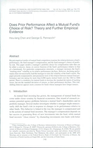
  • 16. 760 Journal of Financial and Quantitative Analysis differences to performance differences as would occur if the same bencbmark were used for all funds.-"^ Figure I sbows the sample's number of G, Gl, and SM mutual funds in oper- ation during each month of our sample period. G funds operating during the past decade account for a majority of our sample observations. The number of funds FIGURE 1 Mutual Fund Sample Population Graph A. Growth Funds 3600 3200 o ) i T ) c > o > 0 > o i O ï o > o a ) O ) < T ] d ï m C î C f i A a > o s o ï O ) Year Graph B Qrowth & Income and Slyle-Mixed Funds 900 700 - ->- 600- 500- 200- 100 ,-,-,-,=n> 03 Oï 05 Year Growth & Income Style-Mixed -''However, in our notiparamelric tesis, we do examitie ihe case of funds' performances relative to the universe of all firms, so thai [he benchmark is effectively the same for all funds.
  • 17. Chen and Pennacchi 761 grew rapidly over the 1990s and peaked approximately three years prior to the sample period's end, since no new funds were added during the last 36 months. This reflects the parameter estimation constraint that a fund report al least three years of returns. The proportions of all G, GI, and SM sample funds that survived (were in operation) as of March 2006 are 67%. 65%. and 62%. respectively. Table 1 presents summary statistics of our mutual fund sample, broken down by fund style. Age is defined as the number of years from the fund's inception date until the date it expired or. for surviving funds, the end-of-sample date of March 2006. Row 1 shows that G and GI funds have, on average, similar ages of approximately 9.9 years, whereas SM funds, whose definition is conditioned on a style change having occurred, are much older. On average, G funds have greater front loads, expense ratios, and turnover ratios than do GI funds. Manager tenure is the average number of years that the same individual or group manages a fund's portfolio. Average manager tenure is similar for G and GI funds, but somewhat greater for SM funds. Table 1 also reports statistics on funds' asset size scores, which measure their relative sizes by assigning a rank score from 0 (smallest) to 1 (largest) for each fund according to its total net asset value at the end of each year. This score is then averaged over each year of the fund's life. The average SM fund is larger than typical GI and G funds, likely a reflection of the greater average age of SM funds. However, on average SM funds display slower but less volatile asset growth, while GI funds grow slightly faster than G funds. The final information in Table 1 relates to a fund's number of share clas.ses and the number of funds in its fund family. These numbers are computed eacb year and then averaged over all years of a fund's life. SM funds tend to have fewer share classes and belong to smaller fund families compared to G and GI funds. VI, Results A. Standard Deviation Ratio Test Results Following prior studies. SDR tests are performed using an annual 2 x 2 clas- sification of whether a fund's return performance over the first six months (RTN) was above (winner) or below (loser) the median and whether its SDR computed over the second versus first halves of the year was above or below the median, where these medians are for all funds in its style class (G. GI. or SM). First, we replicate the tests performed by past research by calculating SDR as in equation (11), equal to the ratio of second to first half-year standard deviations of a fund's total returns. A finding that the frequency of funds in the category (low RTN, high SDR) significantly exceeds 25% would be evidence in favor of the hypothesis that underperforming funds increase their total return standard deviation. Second, we calculate SDR as in equation (16). equal to the ratio of .second to first half-year standard deviations of a fund's returns in excess of benchmark returns (tracking error). The statistical significance of our SDR tests is determined by the method of Busse ((2001). pp. 58, 62-63). His method controls for the auto- and
  • 18. 762 Journal of Financial and Quantitative Analysis TABLE 1 Summary Statistics of Mutual Fund Sample statistics are based on a sample taken ttom thG CRSP Survivor-Bias-Free U.S. Mutual Fund Database covering Ihe period January 1962 lo March 2006 Mutual funds witfi a Wiesentierger or Inveslment Company Data, Inc. (ICDI) objective o( "AggiessivB Growth." "Growth," "Maximum Capiial Gains." "Small Capdaljzation Growth,' or "Long Term Growth," are classilied as growth funds. Mutual tunds with an ob|eclive of "Growth and Income" Of "Growth with Curren! Income" are Classified as growth and income funds. Style-mixed funds are mulual funds with a style of growth or growth and income for only part of their lives Index funds as well as funds with less than 36 consecutive monthly returns are excluded. The sample contains 4.188 growth funds. 861 growth and income funds, and 1,129 style-mixed funds. Age is defined as the number ot years from the fund's inception date until the date it expired or. lor surviving funds, the end-of-sample date of March 2006. A fund's fees and turnover ratios are calculated as the average annual numbers. Managef tenure is the average number of years that an individual manages a fund's portfolio A fund's asset size score is computed by assigning a rank score from 0 (smallest) to 1 (largest) for each fund according to its lotal net asset value at the end of each year. This score IS then averaged over each year ol the tund s life A fund's asset growth equals the average annual log cfiange in total net assets, and (T of a fund's asset growth rates is the time-series standard deviation of annual log changes In total net assets. The number of share classes records for each year the number of funds that have the same fund name but different share classes. Fund family size equals the number of mutual funds that have an identical management oompany name in each year Both fund family size and numbers ol fund share classes are then averaged over each year of a fund's life. Fund No, Of Std. Chaiacietistic Funds Meen Dev. Min. 25% 50% 75% Max. Panel A. Growth Mulual Funds Age (years) 4,188 9.92 6.89 3 6 8 11 74 Front load 4,186 0.014 0.023 0000 0.000 0.000 0.020 0.087 Back toad 4,188 0.011 0.017 0.000 0.000 0,003 0,010 0.060 Expense ratio 4,188 0.016 0.007 0.000 0.011 0.015 0.020 0.167 Turnover ratio 4,145 1.154 2.396 0.000 0.515 0.858 1.363 130.104 Manager tenure (years) 4,011 6.39 3.30 1.00 4.00 6.00 7 75 48.00 Asset size score 4,185 0.41 0.24 0.00 0.21 0.40 0.59 0.97 Asset growth (%) 4,176 32.50 47 00 -277.80 7.39 26.25 50.98 452.18 (T of asset growth (%) 4,138 71.88 56.16 0.22 35.58 56.09 89.69 565.11 Number of share classes 4.188 2.78 139 1 1 3 4 9 Fund family size 4,022 146.74 128.90 1 42 117 224 667 PaneJ S Growth and Income Mulual Ft/nds Age (years) 861 9.94 9.03 3 6 e 11 82 Front load 861 0.011 0.021 0.000 0.000 0.000 O.0O7 0.085 Backktad 861 0.011 0.017 0.000 0000 0.OO2 0.010 0.060 Expense ratio 860 0.014 0.006 0.000 0.009 0.013 0.019 0.035 Turnover ratio 857 0,703 0.508 0.018 0.387 0.611 0.880 5.956 Manager tenure (years) 847 6.31 3 10 2.00 4.33 6.00 7.50 41 00 Asset size score 861 0.42 0.26 0.00 0.21 0.41 0.62 0.99 Asset growth (%) 858 34.35 45.68 -139.95 6.19 27.13 50.62 283.49 (T of asset growth (%) 850 69 95 58.89 0.58 31.93 53.06 85.51 513.00 Number of share classes 861 2.94 1.51 1 2 3 4 9 Fund family size 848 143 11 113.96 1 47 120 212 626 Panel C. Style-Mixed Mutual Funds Age (years) 1.129 16.29 14.50 4 9 13 21 83 Front load 1.129 0.021 0.026 0.000 0000 0.000 0.045 0.085 Back load 1.129 0.007 0.014 0.000 0.000 0.001 0.006 0.050 Expense ratio 1,129 0.014 0.008 0.000 0.009 0.013 0017 0.119 Turnover ratio 1,122 0.905 2.030 0.000 0.413 0.674 1.034 60.996 Manager tenure (years) 1,036 7.85 4.82 200 4,50 6.50 9.00 41.00 Asset size score 1,129 0 49 0.24 0 02 0.30 0.50 0.68 0.98 Asset gfowlh (%) 1,128 21.99 30.98 -174.47 5.42 16,98 34.10 183.41 < of asset growth (%) T 1,126 59.39 43.06 5,32 31.82 48.97 70.52 338.83 Number of share olasses 1,129 1,93 1.24 1 1 1 3 6 Fund family size 1,045 133.34 123.20 1 32 105 199 626 Panel D. All Mulual Funds Age (yeafs) 6,178 11.45 9.61 3 6 9 12 B3 Front load 6,178 0.015 0.023 0.000 O.OOO 0.000 0.030 0.087 Back bad 6,178 0.010 0.017 0.000 0.000 0,002 0.010 0.060 Expense ratio 6,177 0.015 0.007 0.000 0.010 0.014 0.019 0-167 Turnover ratio 6,124 1.045 2 169 0.000 0,469 0.771 1.23B 130 104 Manager tenure (years) 5,894 6.63 3.63 1.00 4.33 6.00 8.00 48.00 Asset size score 6,175 0.43 0.24 0.00 0.22 0,42 0.62 0.99 Asset growth {%) 6,162 30 83 44.50 -277.80 7.02 23 87 47.46 452 18 a of asset grovrth (%) 6,114 69.31 54.59 0.22 34.35 54.14 65,99 565,11 Number ol share olasses 6,178 265 1.42 t 1 3 4 9 Fund family size 5,915 143.85 125.94 1 41 115 216 667
  • 19. Chen and Pennacchi 763 cross-correlation of fund returns that he and GNW (2005) document.^^ It involves simulating fund returns from a Fama-French-Carhart four-factor model for each year and style class to obtain an empirical distribution for the 2 x 2 classifica- tions. Specifically, for each of the 44 years in our sample, we take the Ny funds of a particular style class that operated in year y and regress each of their 12 monthly returns on market, size, book-to-market, and momentum factors. The four factors and regression residuals are arranged into two matrices: a 12 x 4 matrix of the four factors for each month; and a 12 x Ay matrix of the monthly residuals for ^ each fund. To simulate factors, we randomly select a row from the factor matrix and use the following 11 rows in order, continuing with row one of the factor ma- trix after row 12. To simulate residuals, we resample randomly with replacement 12 rows from the residual matrix. We then create simulated monthly returns for A'y artificial funds using the betas and intercepts from the Ny regressions with the simulated factors and simulated residuals.'^^ We compute RTN and SDR (based on either total returns or tracking error) for each artificial fund and allot funds to cells in 2 x 2 contingency tables based on the median fund RTN and the median fund SDR. This procedure is repeated for each year during a particular test sample period (e.g., the entire 1962-2005 sample or the 1995-2005 subsample) to obtain a single simulation. The entire procedure is then repeated 10,000 times to generate an empirical distribution of monthly 2x2 contingency table allotments under the null hypothesis of no tournament behavior. The 10%. 5%, and 1% tails of this empirical distribution provide the significance levels for our SDR tests. Entries in Table 2 are marked by asterisks *. **. and *** when results exceed these respective significance levels in the predicted direction (low RTN, high SDR significantly greater than 25%) and by daggers ^ ^ ^^^ when results are significantly opposite (low RTN. high SDR significantly less than 25%). Panel A of Table 2 reports SDR test results when SDR is based on the stan- dard deviation of total returns as in equation (11), Tests are performed by style class for the entire sample period, 1962-2005, and for four 11-year subsample periods. In addition to these separate tests by fund style, we performed tests by aggregating funds across the style classes. This aggregation was done in two ways: The first "style ranked" (SR) method aggregates funds based their separate style class categorizations. For example, if a fund was categorized as (low RTN, high SDR) based on its particular style class ranking, it remained a (low RTN. high SDR) observation when funds were aggregated across styles to compute aggregate 2 x 2 frequencies. The second "universe ranked" (UR) method aggregates funds of all styles prior to calculating RTN and SDR rankings. Hence, this method es- sentially assumes a tournament where each G, GI. and SM fund competes against all others irrespective of stated style. This aggregation method is consistent with -*'The chi-square tesi of significance used by BHS (1996) is valid only under the assumption that mutual fund returns are serially and cross-sectionally independent. method preserves cross-correlation in the tactor returns and the fund return residuals, as well as most of the autocorrelation in the factors. However, using constant factor loadings throughout the year and resampling Ihe factor retums and fund return residuals removes any relationship between a fund's prior perlbrmance and risk.
  • 20. 764 Journal of Financial and Quantitative Analysis the tests performed in Busse (2001 ) and GNW (2005), which assume that G, GI, and SM funds are a single style. It is clear from Table 2 that there is no evidenee of underperforming funds raising the standard deviation of their total returns in the second half of the year. The only statistically significant results occur for the 1995-2005 period and for the entire 1962-2005 sample period- But these results are exactly opposite to the findings of BHS (1996): Funds that underpertbrmed in the first half of the year tended to reduce the standard deviations of their fund returns in the second TABLE 2 Standard Deviation Ratio Tests of Risk-Taking Behavior Cell frequencies are reported tor a 2 x 2 classification based on a fund's, i) standard deviation ratio (SDR), and ii| relum performance for the lirst six months of each year (RTN). Funds are divided annually into four groups based on whether i) RTN is below (low of "loser") or above (high or "winner") the median, and ii) SDR is above (high) or below (low) the median. In Panel A, risk is defined by the total return standard deviation In Panel B, risk is defined by the standard deviation of tracking error, using as a benchmark the equaiiy weighted return of funds with the same style. Results aggregated across styles are reported m two ways. "All SR" aggregates funds using the previous styie-ranked categonzations ot RTN and SDR: and "All UR" aggregates funds using a uni verse-ranked categorizaiion of RTN and SDR. ', " , and * " indicate 10%, 5%, and 1% two-tailed p-values, respectively, when the frequency of iosers with high SDR is significant in the predicted direction. '', ''*, and " ^ indicate similar signilioance levels for the nonpredicted direction. Significance is calculated for Busses ((2001), pp 62-63) cross-and au to-corr el at ron adjusted test (symbols following low RTN and fiigh SDR entries). Panel A SDR Defined by Ihe Standard Deviation of Tolal Returns Sample Frequency (% of obs.) Low RTN High RTN ("iosers*) ("winners") Low High Low High Type of Funds Obs SDR SDR SDR SDR Samp/e Period. 1962-1972 Growth 1,062 22.88 26.93 26.93 23.26 Growth-Income 221 20.36 28 51 28.51 22.62 Slyle-Miïed 1,226 22.68 27.00 27.00 23.33 AllSFI 2.509 22.56 27,10 27.10 23.24 AilUR 2,609 22.76 27.10 27.10 23.04 Sample Petioa. W73-I983 Growth 1,800 26.11 23.72 23.72 26.44 Growth-Income 282 27.30 21.63 21.63 29.43 Styte-Mixed 1,893 26.04 23.77 23.77 26.41 AilSR 3,975 26.16 23.60 23.60 26.64 AHUR 3,975 27.22 22.74 22.74 27.30 Sample Period: !984-l994 Grovith 4,659 24.10 25.80 25.80 24.30 Growth-Income 812 23.89 25 74 25.74 24.63 Style-Mixed 5,317 25.18 24.77 24,77 25.28 AIISR 10,788 24.62 25 29 25.29 24 81 AMUR 10,78B 24.34 25 63 25.63 24.40 Sample Period: 199&-2005 Growth 27,341 27.93 22.06"' 22.06 27.95 Growth-Income 5,633 27.« 22.51 ^ 22.51 27.55 Style-MiKeb 8,556 27.57 22.39''^ 22.39 27.64 AIISH 41,530 27 76 22.19tt' 22.19 27.83 AIIUR 41,530 28.33 21.66ttt 21.66 28.35 Sample Period: 1962-2005 Growth 34,862 27.17 22 8 0 ^ ' ' 22.B0 27.24 Growth-Income 6,948 26.78 23.0Í 23.04 27.13 Styie-Mixed 16,992 26.30 23.62 f 23.62 26.45 AIISR 58,802 26.87 23 0 6 ^ " 23.06 27.00 AHUR 58.602 27.29 22.69^ 22.69 27.32 (continued on next page)
  • 21. Chen and Pennacchi 765 TABLE 2 (continued) Standard Deviation Ratio Tests of Risk-Taking Behavior Panel B. SDR Defined by the Standard Deviation of Returns in Excess of Benchmark (trackinq error) Sample Frequency 1 % o1 obs.) (• Low RTN High RTN ("losers") ("winners") Low High Low High Type of Funds Obs. SOR SDR SDR SDR Sarriple Perioa: 1962-1972 Growth 1,062 24.20 25.61 25.61 24.58 Growth-Income 221 20.81 28.05" 28,05 23.08 Siyie-Mixed 1,226 24.23 25.45 25.45 24.88 AIISR 2,509 23.91 25.75 25.75 24.59 AHUR 2,509 24.11 25.75 25.75 24,39 Sample Period: 1973-1983 Grow! h 1,800 23.72 26.11" 26.11 24.06 Growth-Income 292 25.89 23.05 23.05 28.01 Slyle-MiJted 1.893 23.45 26.36- 26,36 23.82 AIISR 3,975 23.75 26.01 — 26 01 24.23 AMUR 3,975 23 60 26.36'" 26,36 23.67 Sample Period: 1984-1994 Growth 4.659 23.76 26.14* 26 14 23.95 Growth-Income 812 23.03 26,60 26,60 23.77 Style-Mixed 5,317 24.58 25.37 25,37 24.68 AIISR 10,786 24 11 25.80 25,80 24.30 AHUR 10.788 24 07 25.90 25,90 24.13 Sample Penotí- 1995-2005 Growth 27,341 24.15 25.84— 25.84 2A 17 Growth-Income 5,633 24.69 25.24 25.24 24.Ô2 Siyle-Mixed a,556 24.08 25.89 25.89 24.15 AIISR 41,530 24.21 25.77" 25.77 24.25 AIIUR 41,530 24.22 25.77- 25,77 24.24 Sample Period: I962'2œ5 Growth 34,862 24,07 25.89-" 25.B9 24.15 G towlh-Income 6.948 24,42 25.40 25.40 24.77 Style-Mixed 16.992 24,18 25.75 25.75 24.33 AIISR 58.802 24 15 25.79-" 25.79 24.27 AHUR 58.802 2d,15 25.83— 25.63 24.18 half.-** Our results confirm those of Busse (2001 ) and GNW (2005). who also find evidence contrary to BHS (1996). Panel B of Table 2 reports SDR test results when the SDR is based on the standard deviation of tracking errors as in equation (16). Recall that according to our theory, this type of SDR is the appropriate statistic for testing tournament be- havior. Indeed, we now see that there is substantial evidence that underperforming funds raise the standard deviations of their tracking errors. This behavior is sta- tistically significant over the entire 1962-2005 sample period for G funds and for the aggregation of funds of all styles using either SR or UR rankings. Evidence of our theory's tournament behavior appears for at least some fund styles during '**NoteUial BHS's (1996) SDR lesls used Morningstar dala on the returns of G mutual funds from 1980 lo 1991. When we perfurm SDR lests using our CRSP Jala on the returns of G funds over the exact .siime period. 1980 lo 1991. we match their Undings. Namely, underperforming G funds raise their standard deviations of returns, and this result is slatistically signilicani at the 5'íí' level, even when adjusted for correlation in fund returns. As .shown in Panel A of Table 2. the fact that this significance disappears when different periods of I973-I9S3 or 1984-1994 are tised underscores the fragility of the BHS (1996) findings.
  • 22. 766 Journal of Financial and Quantitative Analysis each of the four subsamples. There is tio contrary evidence of the sort found in Panel A. Measuring risk appropriately as tracking error volatility, rather than total return volatility, appears to make a big difference for tests of tournament behavior. While the results are not tabulated, we followed BHS {1996) by performing SDR tests with samples split by fund age and fund size.^^ Similar to Panel A of Table 2, underperforming funds, both new and old. in addition to small and large, did not raise the standard deviations of their total returns. The only statistically significant results were always in the opposite direction of finding that losing funds decrease their total return standard deviations. However, like Panel B of Table 2. there was evidence that underperforming funds, both new and old, in addition to small and large, raised the standard deviations of their tracking errors as our theory predicts. Evidence for this behavior was strongest for older and larger funds. In summary, these SDR tests provide no evidence for the traditional hypoth- esis that underperformance leads to an increase in the standard deviation of fund returns. In contrast, there is substantially more evidence from SDR tests of an inverse relationship between pertbrmance and the standard deviation of tracking errors. B. Parametric Test Results The previous section's SDR tests are crude in the sense that they allow a fund's risk to change only once per year and that they require a cross-sectional grouping of funds that implicitly assumes these funds engage in similar behavior. We now perform parametric tests for each individual mutual fund that exploits the time-series properties of its returns. These tests permit a fund's risk to change at each observation date and allow risk-taking behavior to differ across funds. Maximum likelihood estimation of the EGARCH equation ( 17), along with either the total returns equation ( 18) or the tracking error equation ( 14), was carried out for the 4,t88 G funds, 861 G! funds, and 1,129 SM funds that had at least 36 monthly observations over the period from January 1962 to March 2006.^*''-^' Table 3 reports summary statistics of the estimates of funds' total return pro- cesses, equations (17) and (18). Recall that this process is not implied by our theoretical model because here, /h¡ represents the standard deviation of a fund's (old} funds were classified as having been in exisleiice for less (greater) than seven years. Small (large) funds were classified as being below (ahove) the median in asset size. -"'We obtained convergence of the likelihood function for greater ihar 99.R% (99.9%) of the fund.^ when estimating the total returns (tracking error) processes. For the few cases where we could nol obtain convergence, the processes were estimated with the GARCH mean reversion coefficient a constrained to equal the median estimate obtained from the other funds for which it was possible to find unconstrained e.stimates. These median values are reported in Tables 3 and 4. " A s a robustness check, we also estimated each fund's total return process (18) and tracking error process ( 14) under the assumption that their means were constants. Specihcally. the equations were estimated, where co and IT, are constant intercept terms. This parametric change had ver>' little effect on the estimates of the other parameters and did not alter the qualitative results that we report below. Results of this alternative specification are available from the authors.
  • 23. Chen and Pennacchi 767 total returns and is permitted to vary with performance, G,. The first five columns of Table 3 give the minimum, first quartile, median, third quartile, and maxinium for each parameter's point estimates for the sample of individual funds. Column 6 reports the proportion of estimates that is strictly greater than zero. Columns 7 and 8 give the proportions of estimates that are significantly positive and nega- tive, respectively, at the 5% confidence level. TABLE 3 Parameter Estimates for Mutual Funds' Return Processes fulaximum likelihood estimates are for the monthly return processes of 4,188 growth, 861 growth-income, and 1,129 style- mined mutual funds hawing at least 36 mcnthly return observations during the January 1962 to fvlarch 2006 sample period. The benchmark returns are the equally weighted returns of all (unds. including funds not having at least 36 observations, within each investment style category, Likefihood function convergence allowed us to obtain estimates of ail parameters for 4,168 growth, 838 growth-income, and 1,129 style-mixed mutual funds. The value of a^ for the remaining growth-income funds was fixed tc the median estimate of the converged growth-income funds, and constrained maximum likelihood estimates of these remaining tunds' other parameters were obtained. r- ^ r- = a o •r 3] ln(/7[_ 1 ) Distribution of Parameler Estimates Summary Statistics Quartiies Proportion of Min. 25% 50% 75% Max, Est > 0 Í > 1.96 f < -1.96 Panel A, Growth Mutual Funds 1' -31,6042 0,0026 0.1313 0.2515 26.5735 0.755 0,288 0.043 äQ ^0.5662 -11,9096 -3.6764 -0.2916 66.6288 0,225 0,074 0.320 3 -5,0833 -1,4663 0.0349 0.9642 5,1631 0,509 0.261 0,199 32 -1,2514 -0 1477 -O.0545 0.0244 6,3555 0.321 0,125 0.245 33 -287.5825 -0,1093 0.1068 0.3474 9.1991 0.631 0.230 0,093 Panel B Growth-Income Mutual Fundí M -4,6868 0.0697 0.2089 0.3221 33.2046 0.849 0.469 0,020 ao -344.1056 -12.5432 -2,7508 0.4794 18.9702 0.271 0,102 0.308 ^1 -379.9965 -1,6006 0.5618 1,3336 6.0008 0,570 0.350 0.189 «2 -80,9025 -0.1239 -0.0183 0.0948 0.6012 0.383 0,189 0.185 03 -157,3799 -0,0149 0,1808 0.3521 4.5886 0,727 0.305 0,102 Panel C Style-MixecJ Mutual Funds f -1.7164 0 0717 0.2214 0.3059 30,6832 0,817 0,563 0.043 ao -36,0890 -10,8326 -2.3014 -0,3614 15.7107 0,214 0.099 0.336 ai -5,5808 -0,8069 0.6350 1,0442 5.0644 0,620 0.425 0.154 az -0,9953 -0,0737 -0,0119 0,0351 0 5067 0.392 0.173 0.202 as -7,6088 0,0071 0,1763 0,3364 3.5623 0,758 0.395 0.081 Pane; D, All Mutual Funds -31.6042 0.0189 0,1598 0 2740 33,2046 0.779 0,364 0,040 ao -344.1056 -11.5747 -3,3073 -0.2627 66.6288 0.229 0 083 0,321 ai -379.9965 -1.2882 0,2227 1.0086 6.0008 0.538 0,304 0.189 33 -80.9025 -0,1294 -O.0350 0,0319 6,3555 0,343 0.U2 0.229 33 -287,5825 -0 0743 0 1371 0,3471 9.1991 0668 0.271 0.092 A positive value for the parameter ui would support the hypothesis that a fund increases its standard deviation of returns as its performance declines. How- ever, the second-to-last row of Table 3 shows that only 34.3% of all mutual funds have a positive estimate for aj and that the median estimate. -0.0350, is negative. Some 14.2% of all funds have a significantly positive estimate of ÍÍ2, but 22.9% have a significantly negative estimate. Hence, more funds appear to lower, rather than raise, the standard deviations of their returns as their performance declines.
  • 24. 768 Journal of Financia! and Quantitative Analysis GI funds are the only .style class that have marginally more estimates of Ü2 that are significantly positive than are significantly negative (18,9% vs. 18,5%). How- ever, the general results of this estimation exercise are consistent with the previous SDR tests in finding relatively few funds that raise the volatility of their returns when their performance is poor. Table 4 presents summary statistics of the estimates of funds' tracking error processes, equations (14) and (17), In this case, sfh, equals the standard devia- tion of a fund's return in excess of its style benchmark return (tracking error), A fund having a positive ai increases its standard deviation of tracking error as its performance declines, which is the type of tournament behavior that is consistent with our theory. As shown in the second-to-last row of Table 4, there are relatively more funds with a significantly positive value of «2 than a significantly negative one (16,8% vs. 12,6%), The result that relatively more funds significantly raise tracking error volatility with poor performance holds for each style category. But clearly this tournament behavior is not widespread. Indeed, the majority of funds have coefficient estimates of «2 that are insignificantly different from zero, and the median point estimate is just slightly below zero. Still, the effect of tournament behavior could be sizeable for many funds. At the third quartile point estimate of «2 = 0,03. a fund that was underperforming by one standard deviation (G, = 0.70) would have an annual standard deviation of tracking error that was 64 basis points (bps) greater than if its performance equaled the benchmark (G, = I).''^ However, a similarly underperforming fund having the first quartile point esti- mate of «2 ~ -0,048 would lower tracking error volatility by 102 bps. Thus, underperformance can lead to economically significant rises or falls in tracking error volatility, depending on the fund. To investigate whether funds that significantly raised tracking error with underperformance (Ö^ > 0) difïer from those that significantly lowered track- ing error with underperformance («2 < 0)., we compared the characteristics of these two groups of funds. Table 5 reports the results of a univariate comparison (Panel A) and a multivariate regression analysis (Panel B), In Panel A. column I gives the total number of funds for which a particular characteristic is rept)rted. and columns 2 and 3 show the numbers of these funds for which we obtained estimates of «2 that were significantly positive and negative, respectively. Then., columns 4 and 5 report the average values of fund characteristics for these two groups of funds whose estimates of 02 were significantly positive and significantly negative, respectively. Column 6 calculates the difference in the two groups" averages, while column 7 reports the /-statistic for the test of whether the group means are statistically different. -''The monthly standard deviation of G, across ail funds and years is Ü.O87 and 0.30, respectivety, on an annual basis. Since from equation (17) dG, 2 the total change in standard deviation at C, = 1 - 0.30 = 0,70 versus G, = I equals 0.7(l 1 1 / I / -ujG-'^dt = - a , I 1 I = 0.214ii2 = 0.0064. 2 ^ 2 - 0.70 )
  • 25. Chen and Pennacchi 769 TABLE 4 Parameter Estimates for Mutual Funds' Excess Return (Tracking Error) Processes Maximum likelihood estimates are for the monthly rettjrn processes o( 4,188 growth. 851 groiMh-income, and 1,129 style- mixed mulual funds having al least 36 montttly return observalions durihg the January 1962 to March 2006 sample period. The benchmark returns are the equally weighted returns ol all lunds, including tunds nol having al leasl 36 oDservations, within each investment style category. Likelihood function convergence allowed us to obtain estimates of ali parameters tor 4,188 growth, 861 growth-income, and!,128 siyie-mixed mutual tunds. The value ol a for the remaining single slyie-mixed lund was tixed lo the median estimate of the converged style-mixed funds, and constrained maximum likelihood estimates tor this remaining ftjnd's other parameters were obtained. = In N(0, (v •32 Distribution of Parameter Estimates Summary Statisties Quartiles Proportion of Est. > 0 I > 1.96 f < -1.96 Panel A. Growiti Mutual Funds -11.3536 -0.0980 0 0079 0 1140 31.2935 0.521 0.095 0.080 -44.2961 -11.1542 -1.654S 0 4566 227.9097 0 296 0 082 0.234 -13.3081 -0.8859 0.7511 1.1768 7.5679 0.644 0.407 0 11! -1.5855 -0.0576 -0.0012 0.0288 0.7814 0 436 0.152 G.I 35 -991.2410 0.0119 0,2866 0.5372 7.8778 0.766 0.377 0064 Panel B. Growth-Income Mutual Funds t'G -10.7731 -0.1200 -0.0171 0 1G32 16.0733 0.443 0.101 0.106 ao -53.8398 -9.4249 -2.2038 0.6581 33 8793 0 294 0.100 0206 -5.2996 -0.5546 0.7961 1.1841 5.8628 0 685 0.419 0.095 -0.7395 -0.0377 -0.0005 0.0223 0.4279 0 453 0.163 0 123 33 -66.5036 0.0177 0.3287 0 5412 17 6268 0.774 0.417 0.079 Panel C. Slyle-Mixed Mutual Funds l^a -2.1955 -0.0958 -0.0059 0.0762 3.0713 0.477 0.090 0.107 -36.6229 -10.2616 -1.5174 0.5645 30.1132 0 291 0.130 0.277 -4.1114 -0.4509 0 8488 1 2268 5.6245 0.693 0.507 0.121 -0,3530 -0.0174 0.0009 0.0362 0.3993 0.521 0 229 0.097 -5.0661 0.0460 0.2402 0.4075 3.7967 0.801 G.5G0 0.078 Panel D. All Mutual Funds -11.3536 -•0 0993 G.OGIO 0 1059 31 2935 0.502 0 095 O.OBB -53.8398 -11.1430 -1.6556 0.4995 227.9097 G.295 0.093 0238 -13.3081 -0.7861 0.7705 1.1847 7 5679 0.659 0 427 Olli -1.5855 -0.0475 -0.0001 0.0298 O.7B14 G.454 0.168 0 126 -991.2410 0.0147 0.2856 0.5088 17.6268 0.773 0 405 0.068 Four of the 11 chiiracteristies are signitieantly different between the two groups. Relative to a fund displaying a positive relationship between performance and tracking error, a fund displaying an inverse relationship (tournament behav- ior) tends to be older, larger, have fewer share classes, and have a portfolio man- ager with a longer tenure at the fund. That older and larger funds appear more prone to tournament behavior is consistent with our (untabulated) SDR test find- ings. However, because many fund characteristics are correlated and may proxy for one another, more insight regarding the determinants of tournament behavior can be obtained through multivariate regression.^-^ -'-'For example, ihe correlation between fund age and manager tenure is 0.4 i across all funds and 0.42 across funds whose estimates of ^2 are statistically significani.