SAP APO Overview

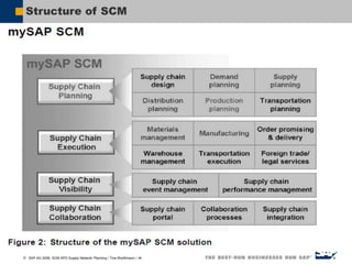
1.  SAP AG 2006, SCM APO Supply Network Planning / Tina Werthmann / ‹#›
Structure of SCM

2.  SAP AG 2006, SCM APO Supply Network Planning / Tina Werthmann / ‹#›
SNC

3.  SAP AG 2006, SCM APO Supply Network Planning / Tina Werthmann / ‹#›
SCM – Demand Planning
Demand planning (DP):
-Demand Planning is a powerful and flexible tool that supports the demand
planning process of an organization
-Its objective is to determine which products are needed for which
customer/location , in which quantity on which date.
-The result of the APO Demand Planning i.e. Forecast is released to Supply
Planning.

4.  SAP AG 2006, SCM APO Supply Network Planning / Tina Werthmann / ‹#›
DP Planning Cycle SEND & Receive
1. Import relevant master and transactional Data
2. Analyze and prepare data
3. Generate Forecast and apply life cycle management
4. Plan promotions and other events
5. Compare and evaluate different scearios
6. Review Final Demand Plan
7. Release final Demand to APO SNP or SAP ERP

5.  SAP AG 2006, SCM APO Supply Network Planning / Tina Werthmann / ‹#›
Basic Terms in DP
5
Info Object
Three types of Basic building blocks of demand planning are possible
• Characteristics
• Key Figures
• Dimensions
Characteristics
Key figures
Dimensions
Logically defined levels at which data can be maintained for planning e.g. Brand,
Country, Product
Numerical fields (Qty and Value) spread across time at which
• Historical data is captured
• Forecasting results are displayed
Logically defined grouping of characteristics for aggregation and disaggregation
InfoCube
InfoCube is a data repository for planning and is typically used to store
• Historical Sales data (Qty., Value)
• Market Research data
• Internal company data (Budgets, Plans)

6.  SAP AG 2006, SCM APO Supply Network Planning / Tina Werthmann / ‹#›
Data Flow
Source System
ex: R/3, BW,
Database,
Legacy System
Data Source InfoProvider
Takes Data and send via INFOPACKAGE
Stores Data in Form of PSA
Data flow via Transformation or DTP

7.  SAP AG 2006, SCM APO Supply Network Planning / Tina Werthmann / ‹#›
Steps to extract the planning data
Generate and export the data source for PA: You can specify which fields you want
the system to use as filters, while extracting data, by checking the selection box.
Replicate the data source : After generating the export Data source, you must
replicate it to create the replica for data extraction and make it available in the data
warehousing workbench for further use.
Create an infocube to store the planning area: To create an infocube for storing
archived planning data, create a basic infocube by running program
/sapapo/ts_parea_to_icube.
Create transformation : When you load data from one SAP BW object such as
datasource into another SAP BW object such as an infocube the data is passed through a
transformation
Create DTP: you use the data transfer process to transfer data within SAP BW from a
persistent object to another object in accordance with certain transformations and filters.
How data from planning area can be stored in infocube via data source, transformation,
DTP and Infopackge

8.  SAP AG 2006, SCM APO Supply Network Planning / Tina Werthmann / ‹#›
Steps in Mass processing
Define Activity
/n/SAPAPO/MC8T to define the
activity
Planning Book
Planning View
Action
Profile
Create Job
/n/SAPAPO/MC8D Create planning
Job
/n/sapapo/MC8E change planning job
Activity
Version
Selection Variants
Aggregation Level
Schedule Job
/n/sapapo/MC8G Schedule Job
Manual release of DP to SNP
/n/sapapo/mc90

9.  SAP AG 2006, SCM APO Supply Network Planning / Tina Werthmann / ‹#›
Capabilities
 Statistical Forecasting
 Selection of advanced statistical tools (Univariant, Multilinear, Composite, etc.)
 Collaborative Planning
 Ability to conduct intra and cross-company Demand Planning collaboration via Internet
 Flexible Multi Level Planning
 Ability to plan at various levels of data hierarchy (product, region)
 Promotion Planning
 Planning, managing and evaluation of the impact of promotions on demand
•Product Life Cycle
 Ability to use phase-in and phase-out profiles and like modeling to manage new products and
obsolescence
•Planning by Exception
 Use of Alerts to report exceptions

10.  SAP AG 2006, SCM APO Supply Network Planning / Tina Werthmann / ‹#›
Forecast Profile
MLR profile : Multilinear regression profile : Casual Analysis on
casual factor such as price budgets and campaigns the system uses
MLR to Calculate the influence of casual factor on past sales.
Univariate are model that investigate historical data according to
constant trend and seasonal pattern and issue forecast error acc.
Composite profile is used to combine multiple forecast into one final
forecast
Statistical forecast: you assign a univariate forecast profile, MLR
profile and composite profile to the master forecast profile to
generate the forecast

11.  SAP AG 2006, SCM APO Supply Network Planning / Tina Werthmann / ‹#›
Demand Planning Structure

12.  SAP AG 2006, SCM APO Supply Network Planning / Tina Werthmann / ‹#›
Demand Planning Configuration
12
• DP and SNP data is divided into
planning areas, and subdivided into
versions.
• Planning Area contains
characteristics, and key figures for
planning, and must be initialized
before planning.
Planning Area
Planning Book
Data View
Characteristic
s
Key Figures
Characteristics
Product
Region
Sales Area
Customer
Key Figures
Actual Sales
Statistical
Forecast
Production
Quantity
Version
000 Active
Version
001 Simulation
Version
MPOS

13.  SAP AG 2006, SCM APO Supply Network Planning / Tina Werthmann / ‹#›
Master Planning Object
Structure
A master planning object structure (MPOS)
contains plannable characteristics for one or
more planning areas
Characteristics determine the levels on which
you can plan and save data
 E.g. If planning is done at Product level then the
MPOS will contain those characteristics.
The existence of an MPOS is a prerequisite for
being able to create a planning area
Generation of CVCs are done within the MPOS
“Aggregates” are defined in the MPOS
13
Master Planning Object Structure
DP Characteristics, SNP Characteristics
Aggregates
Planning Area
Characteristics Key Figures Version
Characteristic Value Combinations
CVC

14.  SAP AG 2006, SCM APO Supply Network Planning / Tina Werthmann / ‹#›
Characteristic Value
Combinations
14
• Characteristic Value Combinations (CVC)
define the relationship between characteristic
values and form the basis for aggregation /
disaggregation of key figure values
• CVC are created in MPOS because it is the
MPOS that contains all the characteristic to
decide at which level planning will be done
• CVC are either created manually or
automatically generated
• It is against these CVC that values in Key
Figure are stored

15.  SAP AG 2006, SCM APO Supply Network Planning / Tina Werthmann / ‹#›
Planning Area
15
Planning Areas are the central data structures for Demand Planning and Supply Network
Planning.
Planning Area
(Characteristics and Key Figures)
General Parameters
• Base Unit of Measure
• Base Currency
• Exchange Rate Type
Storage Buckets Profile
(Defines the time bucket in which data is stored)
• Day
• Week
• Calendar year/month
• Quarter
• Year
• Posting Period
Storage Bucket Profile is a pre-
requisite to have a Planning
Area.

16.  SAP AG 2006, SCM APO Supply Network Planning / Tina Werthmann / ‹#›
Planning Area Version
16
• Versions store data for a
planning area
• To store data for a planning
version, time series must be
created for that version.
• The time series is created in
the Live Cache for each CVC,
and each key figure.
APO Master Data (Model Independent)
Planning Area
Characteristics Key Figures
Active Version 000 Planning Version n
Active Model Simulation Model

17.  SAP AG 2006, SCM APO Supply Network Planning / Tina Werthmann / ‹#›

18.  SAP AG 2006, SCM APO Supply Network Planning / Tina Werthmann / ‹#›

19.  SAP AG 2006, SCM APO Supply Network Planning / Tina Werthmann / ‹#›

20.  SAP AG 2006, SCM APO Supply Network Planning / Tina Werthmann / ‹#›

21.  SAP AG 2006, SCM APO Supply Network Planning / Tina Werthmann / ‹#›
Basic Process in Demand Planning

22.  SAP AG 2006, SCM APO Supply Network Planning / Tina Werthmann / ‹#›

23.  SAP AG 2006, SCM APO Supply Network Planning / Tina Werthmann / ‹#›
 Supply Network Planning results in a feasible, cross-location plan for
production, procurement and distribution. This plan covers the medium-term
planning horizon.
 SNP is not for detailed, but for rough-cut planning, since ...
 only critical products are considered, i.e. products manufactured on
bottleneck resources and products with a long replenishment lead time,
 the smallest time unit in SNP is “day“ (and not second like in PP/DS).
Supply Chain / Supply Network
What is Supply Network Planning (SNP)?

24.  SAP AG 2006, SCM APO Supply Network Planning / Tina Werthmann / ‹#›

25.  SAP AG 2006, SCM APO Supply Network Planning / Tina Werthmann / ‹#›
SNP Master data

26.  SAP AG 2006, SCM APO Supply Network Planning / Tina Werthmann / ‹#›
SNP master data (1)
Quota
arrangements
 Locations (/sapapo/loc3)
 Products (/sapapo/mat1)
 Transportation lanes (/sapapo/scc_tl1)
 Resources (/sapapo/res01)
 PPMs (/sapapo/scc03)
 PDS (/sapapo/curto_simu)
 Quota arrangements (/sapapo/scc_tq1)

27.  SAP AG 2006, SCM APO Supply Network Planning / Tina Werthmann / ‹#›

28.  SAP AG 2006, SCM APO Supply Network Planning / Tina Werthmann / ‹#›
Overview of SNP planning tools - Heuristic
 The SNP heuristic creates a medium-term production and distribution plan for the entire
network (cross-location planning).
 Depending on the procurement type, the heuristic creates planned orders, purchase
requisitions, and stock transport orders to cover demands (forecasts, sales orders and
dependent demand).
 The planning scope of the heuristic depends on which of the three types of heuristic is
executed. The three types of heuristic are:
 Location: Plans all selected products in one selected location
 Network: Plans selected products in all locations
 Multi-level: Plans the selected products including all input products in all locations
 The heuristic does not take into account any constraints or costs, which means that the
plan created will not necessarily be feasible. In a second step after the heuristic run, the
planner can then adjust the plan using capacity-leveling in interactive SNP planning in
order to create a plan that is feasible. Capacity utilization can be checked in interactive
planned (capacity view (SNP94(2)).
 The heuristic can be executed interactively and in the background.
 Checking of results:
 Interactive planning (sapapo/sdp94)
 Product view (sapapo/rrp3)
 Application log (/sapapo/snpaplog)

29.  SAP AG 2006, SCM APO Supply Network Planning / Tina Werthmann / ‹#›
Category

30.  SAP AG 2006, SCM APO Supply Network Planning / Tina Werthmann / ‹#›
Heuristic results
 Heuristic usually generates the following kind of orders:
 Receipts:
 External procurement: Purchase requisition (PurRqs – category AG;
key figure 9APSHIP “Distribution Receipt (Planned)”)
 Inhouse production: SNP:Planned order (SNP:PL-ORD – category EE;
key figure 9APPROD “Production (Planned)”)
 Demands: Stock transport order (PreqRel – category BH;
key figure 9ADMDDI “Distribution Demand (Planned)”)
 In special scenarios (e.g. VMI, scheduling agreements, subcontracting) orders
with different categories are created and different key figures are used.

31.  SAP AG 2006, SCM APO Supply Network Planning / Tina Werthmann / ‹#›

32.  SAP AG 2006, SCM APO Supply Network Planning / Tina Werthmann / ‹#›

33.  SAP AG 2006, SCM APO Supply Network Planning / Tina Werthmann / ‹#›

34.  SAP AG 2006, SCM APO Supply Network Planning / Tina Werthmann / ‹#›

35.  SAP AG 2006, SCM APO Supply Network Planning / Tina Werthmann / ‹#›

36.  SAP AG 2006, SCM APO Supply Network Planning / Tina Werthmann / ‹#›

37.  SAP AG 2006, SCM APO Supply Network Planning / Tina Werthmann / ‹#›

38.  SAP AG 2006, SCM APO Supply Network Planning / Tina Werthmann / ‹#›

39.  SAP AG 2006, SCM APO Supply Network Planning / Tina Werthmann / ‹#›

40.  SAP AG 2006, SCM APO Supply Network Planning / Tina Werthmann / ‹#›

41.  SAP AG 2006, SCM APO Supply Network Planning / Tina Werthmann / ‹#›
Deployment
Fair share= Demand > Supply
PUSH = Demand < Supply

42.  SAP AG 2006, SCM APO Supply Network Planning / Tina Werthmann / ‹#›
Fair share rule A and B

43.  SAP AG 2006, SCM APO Supply Network Planning / Tina Werthmann / ‹#›

44.  SAP AG 2006, SCM APO Supply Network Planning / Tina Werthmann / ‹#›

45.  SAP AG 2006, SCM APO Supply Network Planning / Tina Werthmann / ‹#›

46.  SAP AG 2006, SCM APO Supply Network Planning / Tina Werthmann / ‹#›
Application of production planning

47.  SAP AG 2006, SCM APO Supply Network Planning / Tina Werthmann / ‹#›

48.  SAP AG 2006, SCM APO Supply Network Planning / Tina Werthmann / ‹#›
Factor for SAP PP/DS

49.  SAP AG 2006, SCM APO Supply Network Planning / Tina Werthmann / ‹#›

50.  SAP AG 2006, SCM APO Supply Network Planning / Tina Werthmann / ‹#›

51.  SAP AG 2006, SCM APO Supply Network Planning / Tina Werthmann / ‹#›
PPDS Production Planning Runs
1. SAP_MRP_001- Production planning (high speed) applicable for mass
applications , shortage is shown using alert, This procedure essentially blows
out the MRP by the low-level code (or the top item, then the subcomponents and
so on)= MRP
2. SAP_MRP_002: Product planning does the opposite it plan all top level material
and components at once (aka plan components immediately if a dependent
requirement was created for them in planning the superior product.
An interesting result of this is that because MRP is both Supply
planning and production method, PPDS can create STRs with an
MRP Run which is a PPDS Heuristic SAP_MRP_001,
1. Fair share rule
2. Pull deployment horizon
3. Push deployment horizon
4. Snp Checking Horizon

52.  SAP AG 2006, SCM APO Supply Network Planning / Tina Werthmann / ‹#›
Repetitive Manufacturing Scheduling Heuristic
SAP_DS_01 Stable forward scheduling: Suitable for the explosion of
backlogs or capacity overloads with an unchanged scheduling
sequence. The heuristic can be interactively in the detailed
scheduling planning board and the background in the production
planning run.
Used to resolve planning related interruptions using several BOM
Level(finite)
SAP_PMAN_02: Infinite forward scheduling- Compact forward
scheduling in the event of a scheduling delay in make to
engineering or make to order production based on today’s date or
an entered date.