SlideShare a Scribd company logo
1 of 200
Download to read offline
Conducting Laboratory
Experiments Properly
with Statistical Tools:
An Easy Hands-on Tutorial
Tetsuya Sakai (Waseda University)
tetsuyasakai@acm.org
8th July@SIGIR 2018, Ann Arbor Michigan, USA.
Tutorial materials:
If you want a hands-on experience at the tutorial,
please do the following BEFORE ATTENDING:
- Download
http://waseda.box.com/SIGIR2018tutorial
- Install R on your laptop. Then install the tidyr (for
reformatting data) and pwr libraries (for power
calculation)
If you have reshape2 instead of tidyr and
know how to use melt that’s okay too
Tutorial Outline
• Part I (9:00-10:00)
- Preliminaries
- Paired and two-sample t-tests, confidence intervals
- One-way ANOVA and two-way ANOVA without replication
- Familywise error rate
[Coffee Break (10:00-10:30)]
• Part II (10:30-12:00)
- Tukey’s HSD test, simultaneous confidence intervals
- Randomisation test and randomised Tukey HSD test
- What’s wrong with statistical significance tests?
- Effect sizes, statistical power
- Topic set size design and power analysis
- Summary: how to report your results
IF YOU WANT MORE, PLEASE READ:
Sakai, T.: Laboratory Experiments in Information Retrieval: Sample Sizes, Effect Sizes,
and statistical power, to appear, Springer, 2018.
Which search engine is better?
(paired data)
0.4 0.4
0.8 0.6
0.7 0.5
Some evaluation
measure score
Sample size n = 3
Which search engine is better?
(unpaired data)
0.4
0.8
0.7
1.0
0.8
0.1
0.5
n1 = 3
n2 = 4
Statistical significance testing
[Robertson81, p.23]
“More particularly, having performed a comparison
of two systems on specific samples of documents
and requests, we may be interested in the statistical
significance of the difference, that is in whether the
difference we observe could be simply an accidental
property of the sample or can be assumed to
represent a genuine characteristic of the
populations.”
“Document collection as a sample” [Robertson12] not discussed in this tutorial.
Statistically significant result may not be
practically significant (and vice versa)
“It must nevertheless be admitted that the basis for
applying significance tests to retrieval results is not well
established, and it should also be noted that
statistically significant performance differences may be
too small to be of much operational interest.”
[SparckJones81, Chapter 12, p.243]
Karen Sparck Jones
1935-2007
Roger Needham
1935-2003
What do samples tell us about
population means?
Are they the same?
Parametric tests for comparing means
• In IR experiments, we often compare sample means to
guess if the population means are different.
• We often employ parametric tests (assume specific
population distributions, e.g., normal)
- paired and two-sample t-tests
(Are the m(=2) population means equal?)
- ANOVA (Are the m(>2) population means equal?)
- Tukey HSD test for m(m-1)/2 system pairs
scores
EXAMPLE
(paired data) n topics
m systems
Sample mean for a system
Null hypothesis, test statistic, p-value
• H0: tentative assumption that all
population means are equal
• test statistic: what you compute
from observed data – under H0,
this should obey a known
distribution (e.g. t-distribution)
• p-value: probability of observing
what you have observed (or
something more extreme)
assuming H0 is true
Null hypothesis
test statistic t0
Type I error and statistical power
Reject H0
if p-value <= α
test statistic t0
tinv(φ; α)
Can’t reject H0 Reject H0
H0 is true
systems are equivalent
Correct conclusion
(1-α)
Type I error
α
H0 is false
systems are different
Type II error
β
Correct conclusion
(1-β)
α/2 α/2
Statistical power: ability to
detect real differences
Type II error
Can’t reject H0
if p-value > α
test statistic t0
tinv(φ; α)
Can’t reject H0 Reject H0
H0 is true
systems are equivalent
Correct conclusion
(1-α)
Type I error
α
H0 is false
systems are different
Type II error
β
Correct conclusion
(1-β)
α/2 α/2
Cohen’s five-eighty convention
Can’t reject H0 Reject H0
H0 is true
systems are equivalent
Correct conclusion
(1-α)
Type I error
α
H0 is false
systems are different
Type II error
β
Correct conclusion
(1-β)
Statistical power:
ability to detect
real differencesCohen’s five-eighty convention:
α=5%, 1-β=80% (β=20%)
Type I errors 4 times as serious as Type II errors
The ratio may be set depending on specific situations
Population means and variances
x: a random variable
f(x): probability density function (pdf) of x
The expectation of any function g(x) is:
Population mean: E(x) i.e. expectation of g(x)=x
Population variance:
How does x move around the
population mean?
Law of large numbers
ANY distribution is okay!
If want a good estimate of the population mean,
just take a large sample and compute the sample mean.
Normal distribution
For given μ and σ (>0), the pdf of a normal
distribution is given by:
where
The distribution is denoted by .
Standard normal distribution
Upper 100P% z-value
For any u ~
that satisfies
zinv(0.05)
5%
Properties of the normal distribution
[Sakai18book]
Central Limit Theorem [Sakai18book]
ANY distribution is okay!
Does CLT really hold? Test it with
uniform distributions (1)
n = 1
Does CLT really hold? Test it with
uniform distributions (2)
n = 2
Does CLT really hold? Test it with
uniform distributions (3)
n = 4
Does CLT really hold? Test it with
uniform distributions (4)
n = 8
Already looking quite like a
normal distribution
Variance getting
smaller
Sample variance
V is an unbiased estimator of the population variance
(just as is an unbiased estimator of the population
mean : )
Chi-square distribution
The distribution is denoted by
φ=5
t distribution
The distribution is denoted by t(φ).
φ=5
Two-sided 100P% t-value
For any t ~ t(φ)
that satisfies
2.5% 2.5%
tinv(5; 0.05)
qt returns one-sided
t-values
Basis of the paired t-test [Sakai18book]
t-distribution is like a standard
normal distribution with uncertainty
Compare this with:
population variance
sample variance
Basis of the two-sample t-test
[Sakai18book]
Pooled variance
homoscedasticity
(equal variance)
F distribution
The distribution is denoted by
φ1 =10 φ2 =20
Upper 100P% F-value
For any F ~ F(φ1 , φ2 )
that satisfies 5%
Finv(10, 20; 0.05)
Basis of ANOVA
See “Basis of the two-sample t-test
Tutorial Outline
• Part I (9:00-10:00)
- Preliminaries
- Paired and two-sample t-tests, confidence intervals
- One-way ANOVA and two-way ANOVA without replication
- Familywise error rate
[Coffee Break (10:00-10:30)]
• Part II (10:30-12:00)
- Tukey’s HSD test, simultaneous confidence intervals
- Randomisation test and randomised Tukey HSD test
- What’s wrong with statistical significance tests?
- Effect sizes, statistical power
- Topic set size design and power analysis
- Summary: how to report your results
IF YOU WANT MORE, PLEASE READ:
Sakai, T.: Laboratory Experiments in Information Retrieval: Sample Sizes, Effect Sizes,
and statistical power, to appear, Springer, 2018.
Historically, IR people were
hesitant about the t-test (1)
“since this normality is generally hard to prove for
statistics derived from a request-document
correlation process, the sign test probabilities may
provide a better indicator of system performance
than the t-test” [Salton+68] (p.15)
Historically, IR people were
hesitant about the t-test (2)
“Parametric tests are inappropriate because we do
not know the form of the underlying distribution”
[VanRijsbergen79] (p.136)
“Since the form of the population distributions
underlying the observed performance values is not
known, only weak tests can be applied; for example,
the sign test.” [SparckJones+97]
But actually the t-test is robust to
minor assumption violations
This assumes normality BUT
CLT says ANYTHING can be viewed as normally distributed once averaged over a large sample.
The robustness of the t-test can also be demonstrated using the randomisation test.
Which search engine is better?
(paired data)
0.4 0.4
0.8 0.6
0.7 0.5
Some evaluation
measure score
Sample size n = 3
Paired t-test (1)
x1j : nDCG of System 1 for the j-th topic
x2j: nDCG of System 2 for the j-th topic
Assume that the scores are independent and that
Then for per-topic differences
Paired t-test (2)
Therefore (from Corollary 5)
where
Sample mean Sample variance
Paired t-test (3)
Two-sided test:
H0 : μ1 = μ2 H1 : μ1 ≠ μ2
Under H0 the following should hold:
Two-sided vs one-sided tests: See [Sakai18book] Ch.1
Paired t-test (4)
Under H0 , should hold.
So reject H0 iff
The difference is statistically significant
at the significance criterion α
http://www.f.waseda.jp/tetsuya/20topics3runs.mat.csv
n=20 topics
m=3 systems
Lazy paired t-test with Excel
p-value
two-sided test
paired t-test
Loading 20topics3runs.mat.csv to R
sample means
Paired t-test with R
Compare with the Excel case
Two-sided test
Which search engine is better?
(unpaired data)
0.4
0.8
0.7
1.0
0.8
0.1
0.5
n1 = 3
n2 = 4
Two-sample t-test (1)
x1j : nDCG of System 1 for the j-th topic (n1 topics)
x2j: nDCG of System 2 for the j-th topic (n2 topics)
Assume that the scores are independent and that
Homoscedasticity (equal variance) assumption.
But the t-test is actually quite robust to the assumption
violation. For a discussion on Student’s and Welch’s
t-tests, see [Sakai16SIGIRshort, Sakai18book]
Two-sample t-test (2)
(From Corollary 6)
Pooled variance
Sample means
Two-sample t-test (3)
H0 : μ1 = μ2 H1 : μ1 ≠ μ2
Under H0 the following should hold:
So reject H0 iff
Lazy two-sample t-test with Excel
p-value
two-sided test
Student’s t-test
Two sets of nDCG scores
treated as unpaired data
⇒ a much larger p-value
In practice, if the scores are
paired, use a paired test.
Two-sample (Student’s) t-test with R
Two-sided test
Compare with the Excel case
Confidence intervals for the difference in
population means - paired data (1)
From the paired t-test,
therefore
Confidence intervals for the difference in
population means - paired data (2)
hence
where
100(1-α)% CI:
Margin
of error
Difference in population means
What does a 95% CI mean?
Difference in population means
(a constant)
:
0.05
If you compute
100 different CIs
from 100
different
samples
(i.e. topic sets)
…
About 95 of
the CIs will
capture the
true difference
CIs for the difference in population means
- unpaired data
From the two-sample t-test,
we obtain the following in a similar manner:
where
Computing 95% CIs in practice
(paired data)
We had it already!
To compute
with Excel, use T.INV.2T(α, n-1)
with R: qt(α/2, n-1, lower.tail=FALSE)
Computing 95% CIs in practice
(unpaired data)
We had it already!
To compute
with Excel, use T.INV.2T(α, n1 + n2 - 2)
with R: qt(α/2, n1+n2-2, lower.tail=FALSE)
Tutorial Outline
• Part I (9:00-10:00)
- Preliminaries
- Paired and two-sample t-tests, confidence intervals
- One-way ANOVA and two-way ANOVA without replication
- Familywise error rate
[Coffee Break (10:00-10:30)]
• Part II (10:30-12:00)
- Tukey’s HSD test, simultaneous confidence intervals
- Randomisation test and randomised Tukey HSD test
- What’s wrong with statistical significance tests?
- Effect sizes, statistical power
- Topic set size design and power analysis
- Summary: how to report your results
IF YOU WANT MORE, PLEASE READ:
Sakai, T.: Laboratory Experiments in Information Retrieval: Sample Sizes, Effect Sizes,
and statistical power, to appear, Springer, 2018.
Analysis of Variance
• A typical question ANOVA addresses:
Given observed scores for m systems,
are the m population means all equal or not?
• ANOVA does NOT tell you which system means are
different from others.
• If you are interested in the difference between
every system pair (i.e. obtaining m(m-1)/2 p-values),
conduct an appropriate multiple comparison
procedure, e.g. Tukey HSD test. No need to do
ANOVA before Tukey HSD.
One-way ANOVA, equal group sizes (1)
• Data format:
• Basic assumption:
or
• Question: Are the m population means equal?
unpaired
data, but
equal
group sizes
(e.g. #topics)
homoscedasticity
Generalises the two-sample t-test, and can handle unequal
group sizes as well. See [Sakai18book]
population mean for System i
One-way ANOVA, equal group sizes (2)
Let
Null hypothesis:
⇔
μ2 = μ3 = 0.2
μ = 0.3
μ1 = 0.5
a1 = 0.2
a2 = -0.1 a3 = -0.1
population grand mean i-th system effect
All population means are equal (to μ)
m=3
One-way ANOVA, equal group sizes (3)
Let
Clearly,
sample grand mean System i’s sample mean
Diff between
an individual score
and the grand mean
can be broken down
into…
Diff between
the system mean
and the grand mean
and…
Diff between
the individual score
and the grand mean
One-way ANOVA, equal group sizes (4)
Interestingly, this also holds:
Between-system
sum of squares
Within-system sum of squares
Total sum of squares (variations)
One-way ANOVA, equal group sizes (5)
From a property of the chi-square distribution,
hence
One-way ANOVA, equal group sizes (6)
As for SA , since
Corollary 1 gives us
Hence, under H0 ,
From a property of the chi-square distribution,
under H0.
One-way ANOVA, equal group sizes (7)
Hence, by definition, under H0 ,
Under H0 :
One-way ANOVA, equal group sizes (8)
Under H0 ,
so reject H0 iff
Conclusion: probably
not all population
means are equal
One-way ANOVA with R (1)
Here, just as an exercise, treat the matrix as if it’s unpaired
data (i.e., sample sizes equal but no common topic set)
The sample means (mean nDGG scores) suggest
System1 > System2 > System3.
But is the system effect statistically significant?
One-way ANOVA with R (2)
mat is a 20x3 topic-by-run matrix:
Let’s convert the format for convenience…
One-way ANOVA with R (3)
A 60x2 data.frame Gather all
columns of mat
One-way ANOVA with R (4)
• φA = m-1 = 3-1 = 2
• φE1 = m(n-1) = 3(20-1) = 57
The system effect
is statistically significant
at α = 0.05
p-value
The three systems are probably not all equally effective,
but we don’t know where the difference lies.
Two-way ANOVA without replication (1)
• Data format:
• Basic assumption:
i-th system effect
j-th topic effect
A common
topic set
for all m
systems
(paired data)
Two-way ANOVA without replication (2)
Clearly,
sample grand mean System i’s sample mean
Topic j’s sample mean
Two-way ANOVA without replication (3)
Similarly:
Between-topic
sum of squaresFrom one-way ANOVA
Two-way ANOVA without replication (4)
It can be shown that under H0,
so reject H0 iff
The system effect is
statistically significant at α
All population system
means are equal
Two-way ANOVA without replication (5)
If also interested in the topic effect, under H0
so reject H0 iff
The topic effect is
statistically significant at α
All population topic
means are equal
Two-way ANOVA without
replication with R (1)
Just inserting a column for topic IDs
Two-way ANOVA without
replication with R (2)
Just converting the data format
Gather all
columns of mat
except Topic
A 60x3 data.frame
Two-way ANOVA without
replication with R (3)
• φA = 3-1 = 2
• φB = 20-1 = 19
• φE1 = (3-1)*(20-1)= 38
The system effect
is statistically highly significant
(so is the topic effect)
The three systems are probably not all equally effective,
but we don’t know where the difference lies.
Tutorial Outline
• Part I (9:00-10:00)
- Preliminaries
- Paired and two-sample t-tests, confidence intervals
- One-way ANOVA and two-way ANOVA without replication
- Familywise error rate
[Coffee Break (10:00-10:30)]
• Part II (10:30-12:00)
- Tukey’s HSD test, simultaneous confidence intervals
- Randomisation test and randomised Tukey HSD test
- What’s wrong with statistical significance tests?
- Effect sizes, statistical power
- Topic set size design and power analysis
- Summary: how to report your results
IF YOU WANT MORE, PLEASE READ:
Sakai, T.: Laboratory Experiments in Information Retrieval: Sample Sizes, Effect Sizes,
and statistical power, to appear, Springer, 2018.
Interested in the differences for all system pairs.
So just repeat t-tests m(m-1)/2 times? (1)
The following is the same as repeating t.test with
paired=TRUE for every system pair...
Compare with the
Paired t-test with R slide
... but is NOT the right thing to do.
Interested in the differences for all system pairs.
So just repeat t-tests m(m-1)/2 times? (2)
The following is the same as repeating t.test with
var.equal=TRUE for every system pair...
Compare with the
Two-sample (Student’s) t-test with R slide
This means using Vp rather
than VE1 from one-way
ANOVA
... but is NOT the right thing to do.
Don’t repeat a regular t-test m(m-1)/2
times!
Why? Suppose a restaurant has a wine cellar. It is
known that one in every twenty bottles is sour.
Pick a bottle; the probability
that it is sour is
1/20 = 0.05
(Assume that we have an
infinite number of bottles)
VIN VIN VIN VIN VIN VIN VIN VIN VIN VIN
A customer orders one bottle
A bottle of red
please
The probability that
sour wine is served
to him is 0.05
VIN
A customer orders two bottles
Two bottles
please
The probability that
sour wine is served
to him is
1-P(both bottles are good)
= 1- 0.95^2
= 0.0975
VIN VIN
A customer orders three bottles
Three bottles
please
The probability that
sour wine is served
to him is
1-P(all bottles are good)
= 1- 0.95^3
= 0.1426
VIN VIN VIN
Comparisonwise vs Familywise error rate
(restaurant owner)
• The restaurant is worried not about the probability
of each bottle being sour, but about the probability
of accidentally serving sour wine to the customer
who orders k bottles. The latter probability should
be no larger than (say) 5%.
YOU SERVED ME SOUR WINE
I’M GONNA TWEET ABOUT IT
Comparisonwise vs Familywise error rate
(researcher)
• We should be worried not about the
comparisonwise Type I error rate, but about the
familywise error rate – the probability of making at
least one Type I error among the k=m(m-1)/2 tests.
• Just repeating a t-test k times gives us a familywise
error rate of 1-(1-α)^k if the tests are independent.
e.g. α=0.05, k=10 ⇒ familywise error rate = 40%!
Multiple comparison procedures
[Carterette12][Nagata+97][Sakai18book]
• Make sure that the familywise error rate is no more
than α.
• Stepwise methods: outcome of one hypothesis test
determines what to do next
• Single step methods: test all hypotheses at the
same time – we discuss these only.
- Bonferroni correction (considered obsolete)
- Tukey’s Honestly Significant Difference (HSD) test
- others (e.g. those available in pairwise.t.test)
Bonferroni correction
[Crawley15 ](pp.17-18)
“The old fashioned approach was to use
Bonferroni’s correction: in looking up a
value for Student’s t, you divide your α value
by the number of comparisons you have
done. […] Bonferroni’s correction is very
harsh and will often throw out the baby
with the bathwater. […] The modern
approach is […] to use the wonderfully
named Tukey’s honestly significant
differences”
Or, equivalently,
multiply each p-value
by k
Come back by 10:30!
Tutorial Outline
• Part I (9:00-10:00)
- Preliminaries
- Paired and two-sample t-tests, confidence intervals
- One-way ANOVA and two-way ANOVA without replication
- Familywise error rate
[Coffee Break (10:00-10:30)]
• Part II (10:30-12:00)
- Tukey’s HSD test, simultaneous confidence intervals
- Randomisation test and randomised Tukey HSD test
- What’s wrong with statistical significance tests?
- Effect sizes, statistical power
- Topic set size design and power analysis
- Summary: how to report your results
IF YOU WANT MORE, PLEASE READ:
Sakai, T.: Laboratory Experiments in Information Retrieval: Sample Sizes, Effect Sizes,
and statistical power, to appear, Springer, 2018.
• Instead of conducting a t-test k = m(m-1)/2 times,
consider the maximum difference (best system –
worst system) among the k differences.
• The distribution that the max difference obeys is
called a studentised range distribution. Its upper
100P% value is denoted by
• We compare the k differences against the above
distribution. By construction, if the maximum is not
statistically significant, the other differences are not
statistically significant either. Hence the familywise
error rate can be controlled.
How Tukey HSD works
qtukey(P, m, φ, lower.tail=FALSE) in R
Tukey HSD with equal group sizes (1)
Data structure: same as one-way ANOVA with equal
group sizes
Tukey HSD can handle unequal group sizes as well. See [Sakai18book]
sample mean
for System i
unpaired data
Null hypothesis :
the population means for
systems i and i’ are equal
Test statistic:
Reject iff
Tukey HSD with equal group sizes (2)
R: Tukey HSD with equal group sizes
The data.frame we made for
one-way ANOVA
Only the diff between Systems 1
and 3 statistically significant at
α=0.05
Tukey HSD with paired observations (1)
Data structure: same as two-way ANOVA without
replication
sample mean
for System i
sample mean
for Topic j
paired data
Null hypothesis :
the population means for
systems i and i’ are equal
Test statistic:
Reject iff
Tukey HSD with paired observations (2)
R: Tukey HSD with paired observations
The data.frame we made for two-way
ANOVA without replication
The difference between Systems 1 and 3
and that between Systems 2 and 3 are
statistically highly significant
If you want a 95%CI for the diff between
every system pair…
• If you use the t-test-based MOE for every system
pair, this approach has the same problem as
repeating t-tests multiple times.
• Use a Tukey-based MOE instead to construct a
simultaneous CI – to capture all true means at the
same time, not individually.
Computing the MOE for simultaneous CIs
From Tukey HSD with equal group sizes (unpaired data)
From Tukey HSD with paired observations
Apply the above MOE to each of the k differences
R: Simultaneous 95%CI,
equal group sizes (unpaired data)
MOE = 0.081314
Upper limit = diff + MOELower limit = diff - MOE
R: Simultaneous 95%CI,
paired observations
MOE = 0.033342
(CIs are narrower than the unpaired case)
Upper limit = diff + MOELower limit = diff - MOE
Tutorial Outline
• Part I (9:00-10:00)
- Preliminaries
- Paired and two-sample t-tests, confidence intervals
- One-way ANOVA and two-way ANOVA without replication
- Familywise error rate
[Coffee Break (10:00-10:30)]
• Part II (10:30-12:00)
- Tukey’s HSD test, simultaneous confidence intervals
- Randomisation test and randomised Tukey HSD test
- What’s wrong with statistical significance tests?
- Effect sizes, statistical power
- Topic set size design and power analysis
- Summary: how to report your results
IF YOU WANT MORE, PLEASE READ:
Sakai, T.: Laboratory Experiments in Information Retrieval: Sample Sizes, Effect Sizes,
and statistical power, to appear, Springer, 2018.
Computer-based tests
• Unlike classical significance tests, do not require
assumptions about the underlying distribution
• Bootstrap test [Sakai06SIGIR][Savoy97] – assumes
the observed data are a random sample from the
population. Samples with replacement from the
observed data.
• Randomisation test [Smucker+07] – no random
sampling assumption. Permutes the observed data.
Randomisation test for paired data (1)
Suppose we have an nDCG matrix for
two systems with n topics.
Are these systems equally effective?
Randomisation test for paired data (2)
Suppose we have an nDCG matrix for
two systems with n topics.
Are these systems equally effective?
Let’s assume there is a single hidden
system. For each topic, it generates
two nDCG scores. They are randomly
assigned to the two systems.
Randomisation test for paired data (3)
If H0 is right, these alternative matrices
(obtained by randomly permuting each
row of U) could also have occurred
Randomisation test for paired data (4)
There are 2 possible matrices, but
let’s just consider B of them
(e.g. 10000 trials)
n
Randomisation test for paired data (5)
How likely is the observed difference (or something
even more extreme) under H0? → p-value
Randomisation test for paired data -
pseudocode
The exact p-value changes slightly depending on B.
Random-test in Discpower [Sakai14PROMISE]
http://research.nii.ac.jp/ntcir/tools/discpower-en.html
Contains a tool for
conducting a
randomisation test or
randomised Tukey HSD
test
http://www.f.waseda.jp/tetsuya/20topics2runs.scorematrix
Mean difference and
p-value (compare
with paired t-test)
Paired randomisation test, B=5000 trials
A 20x2 matrix,
white-space-separated
Randomised Tukey HSD test for paired data (1)
Suppose we have an nDCG matrix for
more than two systems with n topics.
Are these systems equally effective?
Suppose we have an nDCG matrix for
more than two systems with n topics.
Which system pairs are really
different?
Randomised Tukey HSD test for paired data (2)
Let’s assume there is a single hidden
system. For each topic, it generates m
nDCG scores. They are randomly
assigned to the m systems.
If H0 is right, these alternative matrices
(obtained by randomly permuting each
row of U) could also have occurred
Randomised Tukey HSD test for paired data (3)
Randomised Tukey HSD test for paired data (4)
There are (m!) possible matrices, but
let’s just consider B of them
(e.g. 10000 trials)
n
How likely are the observed differences
given the null distribution of the maximum differences?
→ Tukey HSD p-value
Randomised Tukey HSD test for paired data (5)
Randomised Tukey HSD – pseudocode
(adapted from [Carterette12])
The exact p-value changes slightly depending on B.
http://www.f.waseda.jp/tetsuya/20topics3runs.scorematrix
Randomised Tukey HSD test, B=5000 trials
Compare the p-values with
those of the Tukey HSD test
with R (paired data)
A 20x3 matrix,
white-space-separated
Tutorial Outline
• Part I (9:00-10:00)
- Preliminaries
- Paired and two-sample t-tests, confidence intervals
- One-way ANOVA and two-way ANOVA without replication
- Familywise error rate
[Coffee Break (10:00-10:30)]
• Part II (10:30-12:00)
- Tukey’s HSD test, simultaneous confidence intervals
- Randomisation test and randomised Tukey HSD test
- What’s wrong with statistical significance tests?
- Effect sizes, statistical power
- Topic set size design and power analysis
- Summary: how to report your results
IF YOU WANT MORE, PLEASE READ:
Sakai, T.: Laboratory Experiments in Information Retrieval: Sample Sizes, Effect Sizes,
and statistical power, to appear, Springer, 2018.
[Bakan66]
“The test of significance does not provide the
information concerning psychological
phenomena characteristically attributed to it;
and a great deal of mischief has been
associated with its use.”
[Deming75]
“Little advancement in the teaching of
statistics is possible, and little hope for
statistical methods to be useful in the frightful
problems that face man today, until the
literature and classroom be rid of terms so
deadening to scientific enquiry as null
hypothesis, population (in place of frame),
true value, level of significance for comparison
of treatments, representative sample.”
[Loftus91]
“Despite the stranglehold that hypothesis
testing has on experimental psychology, I find
it difficult to imagine a less insightful means of
transiting from data to conclusions.”
[Cohen94] (1)
“And we, as teachers, consultants, authors,
and otherwise perpetrators of quantitative
methods, are responsible for the ritualization
of null hypothesis significance testing (NHST; I
resisted the temptation to call it statistical
hypothesis inference testing) to the point of
meaninglessness and beyond. I argue herein
that NHST has not only failed to support the
advances of psychology as a science but also
has seriously impeded it.”
[Cohen94] (2)
“What’s wrong with NHST? Well, among many other
things, it does not tell us what we want to know, and
we so much want to know what we want to know
that, out of desperation, we nevertheless believe
that it does! What we want to know is “Given these
data, what is the probability that H0 is true?” But as
most of us know, what it tells us is “Given that H0 is
true, what is the probability of these (or more
extreme) data?””
p-value = Pr(D+| H)
not Pr(H|D)!
See also
[Carterette15]
[Sakai17SIGIR]
[Rothman98]
“When writing for Epidemiology, you can also
enhance your prospects if you omit tests of statistical
significance. Despite a wide spread belief that many
journals require significance tests for publication, […]
every worthwhile journal will accept papers that
omit them entirely. In Epidemiology, we do not
publish them at all. Not only do we eschew
publishing claims of the presence or absence of
statistical significance, we discourage the use of this
type of thinking in the data analysis [….]”
[Ziliak+08]
“Statistical significance is surely not the only
error in modern science, although it has been,
as we will show, an exceptionally damaging
one.”
“Most important is to minimise Error of the
Third Kind, “the error of undue inattention,”
which is caused by trying to solve a scientific
problem using statistical significance or
insignificance only.”
[Harlow+16]
“The main opposition to NHST then and now
is the tendency for researchers to narrowly
focus on making a dichotomous decision to
retain or reject a null hypothesis, which is
usually not very informative to current or
future research[…] Although there is still not a
universally agreed upon set of practices
regarding statistical inference, there does
seem to be more consistency in agreeing on
the need to move away from an exclusive
focus on NHST […]”
Statistical significance: Problem 1
Many misinterpret and/or misuse significance tests.
American Statistical Association statement (March
2016):
• P-values do not measure the probability that the
studied hypothesis is true, or the probability that
the data were produced by random chance alone.
• A p-value, or statistical significance, does not
measure the size of an effect or the importance of a
result.
p-value = Pr(D+|H)
not Pr(H|D)!
Statistical significance: Problem 2
Dichotomous thinking: statistically significant or not?
(More important questions:
- How much is the difference?
- What does a difference of that magnitude mean to us?)
p=0.049 ⇒ statistically significant at α=0.05
p=0.051 ⇒ NOT statistically significant at α=0.05
Reporting the exact p-value is more informative than
saying “p<0.05” BUT THIS IS STILL NOT SUFFICIENT.
Statistical significance: Problem 3
P-value = f(sample_size, effect_size)
- A large effect size ⇒ a small p-value
- A large sample size ⇒ a small p-value
For example, consider:
From the paired
t-test
Magnitude of the difference
A large effect size (standardised mean difference)
⇒ a large t-value ⇒ a small p-value
A large sample size (topic set size)
⇒ a large t-value ⇒ a small p-value
Anything can be made
statistically significant
by making n large enough!
Tutorial Outline
• Part I (9:00-10:00)
- Preliminaries
- Paired and two-sample t-tests, confidence intervals
- One-way ANOVA and two-way ANOVA without replication
- Familywise error rate
[Coffee Break (10:00-10:30)]
• Part II (10:30-12:00)
- Tukey’s HSD test, simultaneous confidence intervals
- Randomisation test and randomised Tukey HSD test
- What’s wrong with statistical significance tests?
- Effect sizes, statistical power
- Topic set size design and power analysis
- Summary: how to report your results
IF YOU WANT MORE, PLEASE READ:
Sakai, T.: Laboratory Experiments in Information Retrieval: Sample Sizes, Effect Sizes,
and statistical power, to appear, Springer, 2018.
Effect size definition [Cohen88]
“it is convenient to use the phrase “effect size”
to mean “the degree to which the
phenomenon is present in the population,” or
“the degree to which the null hypothesis is
false.” Whatever the manner of
representation of a phenomenon in a
particular research in the present treatment,
the null hypothesis always means that the
effect size is zero.”
Effect size definition [Olejnik+03]
“An effect-size measure is a standardized index
and estimates a parameter that is
independent of sample size and quantifies the
magnitude of the difference between
populations or the relationship between
explanatory and response variable.”
Effect size definition [Kelley+12]
“Effect size is defined as a quantitative
reflection of the magnitude of some
phenomenon that is used for the
purpose of addressing a question of
interest.”
Various effect sizes
• Effect sizes for t-tests (and Tukey HSD):
standardized mean differences (covered in
this lecture)
• Effect sizes for ANOVAs: contribution to the
overall variance: see
[Olejnik+03][Sakai18book] etc. for details
• Other forms of effect sizes: see [Cohen88]
etc.
Paired t-test effect size
Standardised mean difference (diff measured in standard deviation units)
Note that
sample size effect size
Reporting dpaired along with the p-value is more informative than just
reporting the p-value. But dpaired uses the standard deviation of the
differences – works only with the paired t-test.
Hedge’s g (1)
Standardised mean difference for the two-sample
case:
Hedge’s g estimates the above:
Common standard
deviation
Pooled variance
Hedge’s g (2)
From Student’s t-test,
so, since ,
note that
Reporting Hedge’s g along with the p-value is more informative than
just reporting the p-value. See [Sakai18book] for bias correction.
See [Sakai18book] for Cohen’s d
Glass’s Δ (my favourite)
• No homoscedasticity assumption!
• Works for both paired and unpaired data!
• A bias-corrected Δ:
“How much is the difference, when measured in standard deviation units
computed from the control group (i.e., baseline) data that we are familiar with?”
Effect sizes for (randomised)
Tukey HSD
If homoscedasticity is assumed (as in classical Tukey
HSD):
If not, and if there is a common baseline, use Glass’ Δ
by using the standard deviation of that baseline.
Bottom line: report effect sizes as standardised mean differences,
along with p-values.
See “One-way ANOVA,
equal group sizes (8)”
See “Two-way ANOVA
without replication (4)”
Statistical power: ability to detect
real differences
Given α and an effect size that you are interested in
(e.g. standardized mean difference >=0.2),
increasing the sample size n improves statistical power (1-β).
- An overpowered experiment: n larger than necessary
- An underpowered experiment: n smaller than necessary
(cannot detect real differences – a waste of research effort!)
Can’t reject H0 Reject H0
H0 is true
systems are equivalent
Correct conclusion
(1-α)
Type I error
α
H0 is false
systems are different
Type II error
β
Correct conclusion
(1-β)
Tutorial Outline
• Part I (9:00-10:00)
- Preliminaries
- Paired and two-sample t-tests, confidence intervals
- One-way ANOVA and two-way ANOVA without replication
- Familywise error rate
[Coffee Break (10:00-10:30)]
• Part II (10:30-12:00)
- Tukey’s HSD test, simultaneous confidence intervals
- Randomisation test and randomised Tukey HSD test
- What’s wrong with statistical significance tests?
- Effect sizes, statistical power
- Topic set size design and power analysis
- Summary: how to report your results
IF YOU WANT MORE, PLEASE READ:
Sakai, T.: Laboratory Experiments in Information Retrieval: Sample Sizes, Effect Sizes,
and statistical power, to appear, Springer, 2018.
http://sigir.org/files/museum/pub-14/pub_14.pdf
[SparckJones+75]
On TREC topic set sizes [Voorhees09]
“Fifty-topic sets are clearly too small to have
confidence intervals in a conclusion when
using a measure as unstable as P(10). Even for
stable measures, researchers should remain
skeptical of conclusions demonstrated on only
a single test collection.”
TREC 2007 Million Query track [Allan+08] had “sparsely-judged”
1,800 topics, but this was an exception…
Deciding on the number of topics to
create based on statistical
requirements
• Desired statistical power [Webber+08][Sakai16IRJ]
• A cap on the confidence interval width for the mean
difference [Sakai16IRJ]
• Sakai’s Excel tools based on [Nagata03]:
samplesizeTTEST2.xlsx (paired t-test power)
samplesize2SAMPLET.xlsx (two-sample t-test power)
samplesizeANOVA2.xlsx (one-way ANOVA power)
samplesizeCI2.xlsx (paired data CI width)
samplesize2SAMPLECI (two-sample CI width)
Recommendations on topic set
size design tools
• If you’re interested in the statistical power of the
paired t-test, two-sample t-test, or one-way ANOVA,
use samplesizeANOVA2.
• If you’re interested in the CI width of the mean
difference for paired or two-sample data, use
samplesize2SAMPLECI.
• … unless you have an accurate estimate of the
population variance of the score differences
which the paired-data tools
require.
See “Paired t-test (1)”
samplesizeTTEST2
samplesizeCI2
samplesizeANOVA2 input
α: Type I Error probability
β: Type II Error probability, i.e., you want 100(1-β)%
power (see below)
m: number of systems to be compared in one-way
ANOVA
minD: minimum detectable range, i.e.,
whenever the true difference D between
the best and the worst systems is minD
or larger, you want to guarantee 100(1-β)% power
: variance estimate for a particular evaluation
measure (under the homoscedasticity assumption)
μbest
μworst
D
m system means
samplesizeANOVA2:
“alpha=.05, beta=.20” sheet (1)
Enter values in the orange cells (α=5%, β=20%):
m=10, minD=0.1, =0.1
To ensure 80% power (at α=5%) for one-way ANOVA
with any m=10 systems with a minimum detectable
range of 0.1 in terms of a measure whose variance is
0.1, we need n=312 topics. μbest
μworst
D>= 0.1
m system means
samplesizeANOVA2:
“alpha=.05, beta=.20” sheet (2)
Enter values in the orange cells (α=5%, β=20%):
m=2, minD=0.1, =0.1
To ensure 80% power (at α=5%) for one-way ANOVA
with any m=2 systems with a minimum detectable
difference of 0.1 in terms of a measure whose
variance is 0.1, we need n=154 topics. μbest
μworst
D>= 0.1 Two system means
samplesizeANOVA2:
“alpha=.05, beta=.20” sheet (3)
Since one-way ANOVA with m=2 systems is strictly
equivalent to the two-sample t-test [Sakai18book],
To ensure 80% power (at α=5%) for the two-sample
t-test with a minimum detectable difference of 0.1 in
terms of a measure whose variance is 0.1, we need
n=154 topics. μbest
μworst
D>= 0.1 Two system meansThis n can also be regarded as a pessimistic estimate
for the paired data case.
samplesizeANOVA2: how does it work? (1)
[Nagata03][Sakai16IRJ][Sakai18book]
Remember what we do in one-way ANOVA:
we reject H0 (all m means are equal)
iff See “One-way ANOVA,
equal group sizes (8)”
samplesizeANOVA2: how does it work? (2)
So, whether H0 is true or not, the probability of
rejecting H0 is:
If H0 is true, then F0 ~ F(φA, φE1)
and the above = α
Probability of incorrectly
concluding that the system
means are different
samplesizeANOVA2: how does it work? (3)
So, whether H0 is true or not, the probability of
rejecting H0 is:
If H0 is false, then F0 ~ F’(φA, φE1, λ)
and the above = 1-β
statistical power: probability of
correctly concluding that the two
system means are different
A noncentral F
distribution with a
noncentrality
parameter λ
Accumulates squared
system effects
samplesizeANOVA2: how does it work? (4)
If H0 is false, the power can be approximated as:
where
Let’s call it
Formula P
samplesizeANOVA2: how does it work? (5)
Let’s ensure 100(1-β)% power
whenever D >= minD (e.g., 0.1 in
mean nDCG). To do this, we define:
so that Δ >= minΔ holds.
μbest
μworst
D
m system means
minΔ is the worst-case Δ for topic set sizes
samplesizeANOVA2: how does it work? (6)
• λ=nΔ so the worst-case topic set size n can be
estimated very roughly as:
where λ can be approximated using a linear function
of φA for given (α, β).
• Having thus obtained an n, check with Formula P to
see if the desired power is really achieved. If not,
n++. If the power is too high, n--, etc.
• The excel tool does just that.
samplesize2SAMPLECI input
α: Type I Error probability for
100(1-α)% CIs
δ: cap on the CI width for the
difference between two systems
(two-sample data). That is, you
want the width of any CI to be δ
or smaller.
: variance estimate for a
particular evaluation measure
(under the homoscedasticity
assumption)
The n returned by samplesize2SAMPLECI can also be
regarded as a pessimistic estimate for the paired data case.
Difference in population means
(a constant)
:
Width of this CI
Enter values in the orange cells: α=5%, δ=0.1, =0.1
To ensure the CI width of any between-system difference
to be 0.1 or smaller, we need n=309 topics.
samplesize2SAMPLECI:
“approximation” sheet
samplesize2SAMPLECI: how does it work? (1)
[Nagata03][Sakai16IRJ][Sakai18book]
From “CIs for the difference in population means –
unpaird data” we have:
and the CI width is twice the MOE.
We want 2MOE <= δ, but since Vp is a random
variable, we use E(Vp) instead:
samplesize2SAMPLECI: how does it work? (2)
Consider a balanced design, n = n1 = n2 . Then the
above can be approximated as:
Let’s call it Inequality C
samplesize2SAMPLECI: how does it work? (3)
To obtain an initial estimate of n that satisfies the
above, consider the CI for an ideal case where σ is
known:
cf.
Inequality C
Remember, the t-
distribution is like a
standard normal
distribution with
uncertainty
samplesize2SAMPLECI: how does it work? (4)
Hence
• This gives us an optimistic estimate of n,
so check with Inequality C. If the condition is not
satisfied, n++, etc.
• The excel tool does just that.
Estimating the common variance
If you have a topic-by-system score matrix or two
from some pilot data,
an unbiased estimator can be
obtained as:
Pooled estimate
Estimate from one matrix See “Two-way ANOVA without replication (4)”
A score matrix from
test collection C
Some real estimates based on TREC
data (using VE1 rather than VE2)
See “One-way ANOVA, equal group sizes (8)”
Some measures are less stable ⇒ require larger topic set sizes under the same requirement
Some topic set size design results
[Sakai18book]
The paired t-test tool does not return tight estimates due to my crude estimate
(covariance not considered)
So, to build a test collection…
1. Build a small data set first (or borrow one from a past
task similar to your own).
2. Decide on a primary evaluation measure, and create
a small topic-by-system score matrix with the small
data set.
3. Compute as VE1 or VE2 and use a topic set size
design tool to decide on n.
4. You can advertise your test collection as follows:
“We created 70 topics, which, according to topic set size
design with = 0.044, is more than sufficient for
achieving 80% power with a (paired) t-test whenever the
true difference in Mean nDCG@10 is 0.10 or larger.”
See previous two slides
Power analysis with R scripts
[Sakai16SIGIR] (adapted from [Toyoda09])
• Given an adequately reported significance test
result in a paper,
- compute the effect size and the achieved power in
that experiment.
- propose a new sample size to achieve a desired
power.
Relies on the pwr library of R
The five R power analysis scripts
[Sakai16SIGIR]
• future.sample.paired (for paired t-tests)
• future.sample.unpairedt (for two-sample t-tests)
• future.sample.1wayanova (for one-way ANOVAs)
• future.sample.2waynorep (for two-way ANOVAs
without replication)
• future.sample.2wayanova2 (for two-way ANOVAs)
future.sample.pairedt
Basically just enter t0 and the actual sample size
OUTPUT:
- Effect size dpaired
- Achieved power of the experiment
- future sample size for achieving 80% power
future.sample.pairedt: an actual
example from a SIGIR paper
A highly underpowered experiment.
In future, use 244 topics, not 28, to achieve 80%
power for this small effect (dpaired = 0.18).
Only 15% power!
Underpowered experiments can be a waste of research effort:
there’s a high chance that you will miss a true difference!
about 85%
future.sample.2waynorep
Basically just enter F0, the number of systems m
and the actual sample size
OUTPUT:
- A partial effect size [Sakai18book]
- Achieved power of the experiment
- future sample size for achieving 80% power
future.sample.2waynorep: an actual
example from a SIGIR paper
A highly underpowered experiment.
In future, use 75 topics, not 17, to achieve 80%
power for this small effect.
Only 18% power!
Underpowered experiments can be a waste of research effort:
there’s a high chance that you will miss a true difference!
about 82%
From [Sakai16SIGIR]
Underpowered/Overpowered
experiments: t-tests
Underpowered/Overpowered
experiments: ANOVAs
Tutorial Outline
• Part I (9:00-10:00)
- Preliminaries
- Paired and two-sample t-tests, confidence intervals
- One-way ANOVA and two-way ANOVA without replication
- Familywise error rate
[Coffee Break (10:00-10:30)]
• Part II (10:30-12:00)
- Tukey’s HSD test, simultaneous confidence intervals
- Randomisation test and randomised Tukey HSD test
- What’s wrong with statistical significance tests?
- Effect sizes, statistical power
- Topic set size design and power analysis
- Summary: how to report your results
IF YOU WANT MORE, PLEASE READ:
Sakai, T.: Laboratory Experiments in Information Retrieval: Sample Sizes, Effect Sizes,
and statistical power, to appear, Springer, 2018.
Reporting a paired t-test result (1)
Clearly state the sample
size within the table!
Clearly indicate what the
numbers are! Which
evaluation measure?
Are they mean values?
Reporting a paired t-test result (2)
“We conducted a paired t-test for the difference
between our proposed system and the baseline in
terms of mean nDCG over n=20 topics. The
difference is not statistically significant (t(19) =
1.3101, p=0.2058, 95%CI[-0.0134, 0.0581]), with the
effect size dpaired = t0/√n = 0.2929.”
Provide as much information as
possible for future researchers.
There are several types of effect
sizes. Clarify which one you are
talking about.
Reporting a two-sample t-test result (1)
Clearly indicate what the
numbers are! Which
evaluation measure?
Are they mean values?
Clearly state the sample
sizes within the table!
Reporting a two-sample t-test result (2)
“We conducted a Student’s t-test for the difference
between the our proposed system (sample size n1 =
20) and the baseline (sample size n2 = 20) in terms of
mean nDCG. The difference is not statistically
significant (t(38) = 0.6338, p=0.53,
95%CI[-0.0491, 0.0938]), with Hedge’s g = 0.2004.”
Note that
If you used Welch’s t-test [Sakai16SIGIRshort], you consciously avoided the
homoscedasticity assumption, so I recommend using Glass’ Δ, not Hedge’s d.
Reporting a (randomised) Tukey
HSD result (1)
Reporting a (randomised) Tukey
HSD result (2)
“We conducted a randomised Tukey HSD test with
B=5,000 trials to compare every system pair […] It
can be observed that System 3 statistically
significantly underperforms Systems 1 (p≒0.0000)
and 2 (p=0.0024). Moreover, we computed an effect
size ESE2 [Sakai18book] for each system pair. It can be
observed that Systems 1 and 3 are almost two
standard deviations apart from each other.”
Also visualise each system’s performance using graphs with error bars,
or boxplots! State clearly what the error bars represent (e.g., 95% CIs)!
Summary
• To design a test collection, use some pilot data to
estimate the variance of a particular evaluation
measure for sample size considerations.
• To design an experiment, use a pilot or existing
study for sample size considerations to ensure
sufficient statistical power. Underpowered
experiments can be a waste of research effort.
• When reporting on statistical significance test
results, report the sample sizes, test statistics,
degrees of freedom, p-values (not the stars
*/**/***), and effect sizes!
Despite what R outputs, it is wrong to decide on α AFTER looking at the results
(e.g. “this difference is statistically significant at α=1% while that is significant at α=5%”)
[Sakai18book]
Thank you for staying
until the end!
References: A-B
[Allan+08] Allan, J., Carterette, B., Aslam, J.A., Pavlu,
V., Dachev, B., and Kanoulas, E.: Million Query Track
2007 Overview, Proceedings of TREC 2007, 2008.
[Bakan66] Bakan, D.: The Test of Significance in
Psychological Research, Psychological Bulletin, 66(6),
pp.423-437, 1966.
References: C-D
[Carterette12] Carterette, B.: Multiple Testing in Statistical
Analysis of Systems-based Information Retrieval Experiments,
ACM TOIS 30(1), 2012.
[Carterette15] Carterette, B.: Bayesian Inference for
Information Retrieval Evaluation, ACM ICTIR 2015, pp.31-40,
2015.
[Cohen88] Cohen, J.: Statistical Power Analysis for the
Behavioral Sciences (Second Edition), Psychology Press, 1988.
[Cohen94] Cohen, J.: The Earth is Round (p<.05), American
Psychologist, 49(12), pp.997-1003, 1994.
[Crawley15] Crawly, M.J.: Statistics: An Introduction Using R
(Second Edition), Wiley, 2015.
[Deming75] Deming, W.E., On Probability as a Basic for Action,
American Statistician, 29(4), pp.146-152, 1975.
References: G-H
[Good05] Good, P.: Permutation, Parametric, and
Bootstrap Tests of Hypothesis (Third Edition),
Springer, 2005.
[Harlow+16] Harlow, L.L., Mulaik, S.A., and Steiger,
J.H.: What If There Were No Significance Tests?
(Classic Edition), Routledge, 2016.
References: K-L
[Kelley+12] Kelly, K. and Preacher, K.J.: On Effect Size,
Psychological Methods, 17(2), pp.137-152, 2012.
[Loftus91] On the Tyranny of Hypothesis Testing in
the Social Sciences, Contemporary Psychology, 36(2),
pp.102-105, 1991.
References: N-O
[Nagata+97] Nagata, Y. and Yoshida, M.: Introduction
to Multiple Comparison Procedures (in Japanese),
Scientist press, 1997.
[Nagata03] Nagata, Y.: How to Design the Sample Size
(in Japanese), Asakura Shoten, 2003.
[Olejnik+03] Olejnik, S. and Algina, J.: Generalized Eta
and Omega Squared Statistics: Measures of Effect
Size for Some Common Research Designs,
Psychological Research, 8(4), pp.434-447, 2003.
References: R
[Robertson81] Robertson, S.E.: The Methodology of
Information Retrieval Experiment, In Sparck Jones, K.
(ed.): Information Retrieval Experiment, Chapter 1,
Butterworths, 1981.
[Robertson12] Robertson, S.E., Kanoulas, E.: On Per-
topic Variance in IR Evaluation, ACM SIGIR 2012,
pp.891-900, 2012.
[Rothman98] Rothman, K.J.: Writing for Epidemiology,
Epidemiology, 9(3), pp.333-337, 1998.
References: S
[Sakai06SIGIR] Sakai, T.: Evaluating Evaluation Metrics based on the Bootstrap, ACM SIGIR 2006,
pp.525-532, 2006.
[Sakai14PROMISE] Sakai, T.: Metrics, Statistics, Tests, PROMISE Winter School 2013: Bridging
between Information Retrieval and Databases (LNCS 8173), Springer, 2014.
[Sakai16IRJ] Topic Set Size Design, Information Retrieval, 19(3), pp.256-283, 2016.
[Sakai16SIGIR] Sakai, T.: Statistical Significance, Power, and Sample Sizes: A Systematic Review of
SIGIR and TOIS, 2006-2015, Proceedings of ACM SIGIR 2016, pp.5-14, 2016.
[Sakai16SIGIRshort] Sakai, T.: Two Sample T-tests for IR Evaluation: Student or Welch?, Proceedings
of ACM SIGIR 2016, pp.1045-1048, 2016.
[Sakai17SIGIR] Sakai, T.: The Probability That Your Hypothesis Is Correct, Credible Intervals, and
Effect Sizes for IR Evaluation, Proceedings of ACM SIGIR 2017, pp.25-34, 2017.
[Sakai18book] Sakai, T.: Laboratory Experiments in Information Retrieval: Sample Sizes, Effect Sizes,
and statistical power, to appear, Springer, 2018.
[Salton+68] Salton, G. and Lesk, M.E.: Computer Evaluation of indexing and text processing, Journal
of the ACM, 15, pp.8-36, 1968.
References: S (continued)
[Savoy97] Savoy, J.: Statistical Inference in Retrieval Effectiveness
Evaluation, Information Processing and Management, 33(4),
pp.495-512, 1997.
[Smucker+07] Smucker, M.D., Allan, J. and Carterette, B.: A
Comparison of Statistical Significance Tests for Information Retrieval
Evaluation, CIKM 2007, pp.623-632, 2007.
[SparckJones+75] Sparck Jones, K. and van Rijsbergen, C.J.: Report
on the Need for and Provision of an ‘Ideal’ Information Retrieval
Test Collection, Computer Laboratory, University of Cambridge,
British Library Research and Development Report No.5266, 1975.
[SparckJones81] Sparck Jones, K. (ed.): Information Retrieval
Experiment, Butterworths, 1981.
[SparckJones+97] Sparck Jones, K. and Willet, P.: Readings in
Information Retrieval, Morgan Kaufmann, 1997.
References: T
[Toyoda09] Toyoda, H.: Introduction to Statistical
Power Analysis: A Tutorial with R (in Japanese), Toyo
Tosyo, 2009.
References: V-W
[VanRijsbergen79] Van Rijsbergen, C.J., Information
Retrieval, Chapter 7, Butterworths, 1979.
[Voorhees09] Voorhees, E.M.: Topic Set Size Redux,
Proceedings of ACM SIGIR 2009, pp.806-807, 2009.
[Webber+08] Webber, W., Moffat, A., and Zobel, J.:
Statistical Power in Retrieval Experimentation,
Proceedings of CIKM 2008, pp.571-580, 2008.
References: Z
[Ziliak+08] The Cult of Statistical Significance: How
the Standard Error Costs Us Jobs, Justice, and Lives,
The University of Michigan Press, 2008.

More Related Content

What's hot

Multinomial Logistic Regression Analysis
Multinomial Logistic Regression AnalysisMultinomial Logistic Regression Analysis
Multinomial Logistic Regression AnalysisHARISH Kumar H R
 
Data Science interview questions of Statistics
Data Science interview questions of Statistics Data Science interview questions of Statistics
Data Science interview questions of Statistics Learnbay Datascience
 
Temporal Networks of Human Interaction
Temporal Networks of Human InteractionTemporal Networks of Human Interaction
Temporal Networks of Human InteractionPetter Holme
 
Churn customer analysis
Churn customer analysisChurn customer analysis
Churn customer analysisDr.Bechoo Lal
 
Community Of Practice Powerpoint Presentation Slides
Community Of Practice Powerpoint Presentation SlidesCommunity Of Practice Powerpoint Presentation Slides
Community Of Practice Powerpoint Presentation SlidesSlideTeam
 
Basic Descriptive Statistics
Basic Descriptive StatisticsBasic Descriptive Statistics
Basic Descriptive Statisticssikojp
 
Machine learning ~ Forecasting
Machine learning ~ ForecastingMachine learning ~ Forecasting
Machine learning ~ ForecastingShaswat Mandhanya
 
NEUROMARKETING - Dissertation (English version, presentation only)
NEUROMARKETING - Dissertation (English version, presentation only)NEUROMARKETING - Dissertation (English version, presentation only)
NEUROMARKETING - Dissertation (English version, presentation only)Valentin Oliver
 
Logistic regression
Logistic regressionLogistic regression
Logistic regressionsaba khan
 

What's hot (20)

Multinomial Logistic Regression Analysis
Multinomial Logistic Regression AnalysisMultinomial Logistic Regression Analysis
Multinomial Logistic Regression Analysis
 
Data Science interview questions of Statistics
Data Science interview questions of Statistics Data Science interview questions of Statistics
Data Science interview questions of Statistics
 
Statistics
StatisticsStatistics
Statistics
 
Hypothesis testing
Hypothesis testingHypothesis testing
Hypothesis testing
 
Temporal Networks of Human Interaction
Temporal Networks of Human InteractionTemporal Networks of Human Interaction
Temporal Networks of Human Interaction
 
Model selection
Model selectionModel selection
Model selection
 
Churn customer analysis
Churn customer analysisChurn customer analysis
Churn customer analysis
 
Predicting the e-commerce churn
Predicting the e-commerce churnPredicting the e-commerce churn
Predicting the e-commerce churn
 
Review of Statistics
Review of StatisticsReview of Statistics
Review of Statistics
 
Community Of Practice Powerpoint Presentation Slides
Community Of Practice Powerpoint Presentation SlidesCommunity Of Practice Powerpoint Presentation Slides
Community Of Practice Powerpoint Presentation Slides
 
Session 7 data analysis
Session 7 data analysisSession 7 data analysis
Session 7 data analysis
 
Descriptive statistics
Descriptive statisticsDescriptive statistics
Descriptive statistics
 
Basic Descriptive Statistics
Basic Descriptive StatisticsBasic Descriptive Statistics
Basic Descriptive Statistics
 
Machine learning ~ Forecasting
Machine learning ~ ForecastingMachine learning ~ Forecasting
Machine learning ~ Forecasting
 
Coefficient of Variation
Coefficient of VariationCoefficient of Variation
Coefficient of Variation
 
Chi square
Chi squareChi square
Chi square
 
Data Analysis
Data AnalysisData Analysis
Data Analysis
 
NEUROMARKETING - Dissertation (English version, presentation only)
NEUROMARKETING - Dissertation (English version, presentation only)NEUROMARKETING - Dissertation (English version, presentation only)
NEUROMARKETING - Dissertation (English version, presentation only)
 
Logistic regression
Logistic regressionLogistic regression
Logistic regression
 
Ch08 ci estimation
Ch08 ci estimationCh08 ci estimation
Ch08 ci estimation
 

Similar to Conducting Statistical Experiments Hands-On

ecir2019tutorial-finalised
ecir2019tutorial-finalisedecir2019tutorial-finalised
ecir2019tutorial-finalisedTetsuya Sakai
 
Designing Test Collections for Comparing Many Systems
Designing Test Collections for Comparing Many SystemsDesigning Test Collections for Comparing Many Systems
Designing Test Collections for Comparing Many SystemsTetsuya Sakai
 
Analyzing experimental research data
Analyzing experimental research dataAnalyzing experimental research data
Analyzing experimental research dataAtula Ahuja
 
Analyzing experimental research data
Analyzing experimental research dataAnalyzing experimental research data
Analyzing experimental research dataAtula Ahuja
 
SPSS statistics - get help using SPSS
SPSS statistics - get help using SPSSSPSS statistics - get help using SPSS
SPSS statistics - get help using SPSScsula its training
 
Spsshelp 100608163328-phpapp01
Spsshelp 100608163328-phpapp01Spsshelp 100608163328-phpapp01
Spsshelp 100608163328-phpapp01Henock Beyene
 
Day 12 t test for dependent samples and single samples pdf
Day 12 t test for dependent samples and single samples pdfDay 12 t test for dependent samples and single samples pdf
Day 12 t test for dependent samples and single samples pdfElih Sutisna Yanto
 
jhghgjhgjhgjhfhcgjfjhvjhjgjkggjhgjhgjhfjgjgfgfhgfhg
jhghgjhgjhgjhfhcgjfjhvjhjgjkggjhgjhgjhfjgjgfgfhgfhgjhghgjhgjhgjhfhcgjfjhvjhjgjkggjhgjhgjhfjgjgfgfhgfhg
jhghgjhgjhgjhfhcgjfjhvjhjgjkggjhgjhgjhfjgjgfgfhgfhgUMAIRASHFAQ20
 
Week 5 Lecture 14 The Chi Square TestQuite often, patterns of .docx
Week 5 Lecture 14 The Chi Square TestQuite often, patterns of .docxWeek 5 Lecture 14 The Chi Square TestQuite often, patterns of .docx
Week 5 Lecture 14 The Chi Square TestQuite often, patterns of .docxcockekeshia
 
Statistics pres 3.31.2014
Statistics pres 3.31.2014Statistics pres 3.31.2014
Statistics pres 3.31.2014tjcarter
 
Week 5 Lecture 14 The Chi Square Test Quite often, pat.docx
Week 5 Lecture 14 The Chi Square Test Quite often, pat.docxWeek 5 Lecture 14 The Chi Square Test Quite often, pat.docx
Week 5 Lecture 14 The Chi Square Test Quite often, pat.docxcockekeshia
 
T test, independant sample, paired sample and anova
T test, independant sample, paired sample and anovaT test, independant sample, paired sample and anova
T test, independant sample, paired sample and anovaQasim Raza
 
Designing Test Collections That Provide Tight Confidence Intervals
Designing Test Collections That Provide Tight Confidence IntervalsDesigning Test Collections That Provide Tight Confidence Intervals
Designing Test Collections That Provide Tight Confidence IntervalsTetsuya Sakai
 

Similar to Conducting Statistical Experiments Hands-On (20)

ecir2019tutorial-finalised
ecir2019tutorial-finalisedecir2019tutorial-finalised
ecir2019tutorial-finalised
 
WSDM2019tutorial
WSDM2019tutorialWSDM2019tutorial
WSDM2019tutorial
 
ecir2019tutorial
ecir2019tutorialecir2019tutorial
ecir2019tutorial
 
Designing Test Collections for Comparing Many Systems
Designing Test Collections for Comparing Many SystemsDesigning Test Collections for Comparing Many Systems
Designing Test Collections for Comparing Many Systems
 
ICTIR2016tutorial
ICTIR2016tutorialICTIR2016tutorial
ICTIR2016tutorial
 
Analyzing experimental research data
Analyzing experimental research dataAnalyzing experimental research data
Analyzing experimental research data
 
Analyzing experimental research data
Analyzing experimental research dataAnalyzing experimental research data
Analyzing experimental research data
 
SPSS statistics - get help using SPSS
SPSS statistics - get help using SPSSSPSS statistics - get help using SPSS
SPSS statistics - get help using SPSS
 
Spsshelp 100608163328-phpapp01
Spsshelp 100608163328-phpapp01Spsshelp 100608163328-phpapp01
Spsshelp 100608163328-phpapp01
 
Day 12 t test for dependent samples and single samples pdf
Day 12 t test for dependent samples and single samples pdfDay 12 t test for dependent samples and single samples pdf
Day 12 t test for dependent samples and single samples pdf
 
jhghgjhgjhgjhfhcgjfjhvjhjgjkggjhgjhgjhfjgjgfgfhgfhg
jhghgjhgjhgjhfhcgjfjhvjhjgjkggjhgjhgjhfjgjgfgfhgfhgjhghgjhgjhgjhfhcgjfjhvjhjgjkggjhgjhgjhfjgjgfgfhgfhg
jhghgjhgjhgjhfhcgjfjhvjhjgjkggjhgjhgjhfjgjgfgfhgfhg
 
Experimental
ExperimentalExperimental
Experimental
 
Week 5 Lecture 14 The Chi Square TestQuite often, patterns of .docx
Week 5 Lecture 14 The Chi Square TestQuite often, patterns of .docxWeek 5 Lecture 14 The Chi Square TestQuite often, patterns of .docx
Week 5 Lecture 14 The Chi Square TestQuite often, patterns of .docx
 
T test
T test T test
T test
 
SIGIR2016
SIGIR2016SIGIR2016
SIGIR2016
 
Statistics pres 3.31.2014
Statistics pres 3.31.2014Statistics pres 3.31.2014
Statistics pres 3.31.2014
 
Week 5 Lecture 14 The Chi Square Test Quite often, pat.docx
Week 5 Lecture 14 The Chi Square Test Quite often, pat.docxWeek 5 Lecture 14 The Chi Square Test Quite often, pat.docx
Week 5 Lecture 14 The Chi Square Test Quite often, pat.docx
 
T test, independant sample, paired sample and anova
T test, independant sample, paired sample and anovaT test, independant sample, paired sample and anova
T test, independant sample, paired sample and anova
 
Designing Test Collections That Provide Tight Confidence Intervals
Designing Test Collections That Provide Tight Confidence IntervalsDesigning Test Collections That Provide Tight Confidence Intervals
Designing Test Collections That Provide Tight Confidence Intervals
 
Introduction to spss
Introduction to spssIntroduction to spss
Introduction to spss
 

More from Tetsuya Sakai

More from Tetsuya Sakai (20)

NTCIR15WWW3overview
NTCIR15WWW3overviewNTCIR15WWW3overview
NTCIR15WWW3overview
 
sigir2020
sigir2020sigir2020
sigir2020
 
ipsjifat201909
ipsjifat201909ipsjifat201909
ipsjifat201909
 
sigir2019
sigir2019sigir2019
sigir2019
 
assia2019
assia2019assia2019
assia2019
 
ntcir14centre-overview
ntcir14centre-overviewntcir14centre-overview
ntcir14centre-overview
 
evia2019
evia2019evia2019
evia2019
 
Evia2017unanimity
Evia2017unanimityEvia2017unanimity
Evia2017unanimity
 
Evia2017assessors
Evia2017assessorsEvia2017assessors
Evia2017assessors
 
Evia2017dialogues
Evia2017dialoguesEvia2017dialogues
Evia2017dialogues
 
Evia2017wcw
Evia2017wcwEvia2017wcw
Evia2017wcw
 
sigir2017bayesian
sigir2017bayesiansigir2017bayesian
sigir2017bayesian
 
NL20161222invited
NL20161222invitedNL20161222invited
NL20161222invited
 
AIRS2016
AIRS2016AIRS2016
AIRS2016
 
Nl201609
Nl201609Nl201609
Nl201609
 
ictir2016
ictir2016ictir2016
ictir2016
 
On Estimating Variances for Topic Set Size Design
On Estimating Variances for Topic Set Size DesignOn Estimating Variances for Topic Set Size Design
On Estimating Variances for Topic Set Size Design
 
Topic Set Size Design with the Evaluation Measures for Short Text Conversation
Topic Set Size Design with the Evaluation Measures for Short Text ConversationTopic Set Size Design with the Evaluation Measures for Short Text Conversation
Topic Set Size Design with the Evaluation Measures for Short Text Conversation
 
assia2015sakai
assia2015sakaiassia2015sakai
assia2015sakai
 
Short Text Conversation@NTCIR-12 Kickoff
Short Text Conversation@NTCIR-12 KickoffShort Text Conversation@NTCIR-12 Kickoff
Short Text Conversation@NTCIR-12 Kickoff
 

Recently uploaded

SAP Build Work Zone - Overview L2-L3.pptx
SAP Build Work Zone - Overview L2-L3.pptxSAP Build Work Zone - Overview L2-L3.pptx
SAP Build Work Zone - Overview L2-L3.pptxNavinnSomaal
 
Developer Data Modeling Mistakes: From Postgres to NoSQL
Developer Data Modeling Mistakes: From Postgres to NoSQLDeveloper Data Modeling Mistakes: From Postgres to NoSQL
Developer Data Modeling Mistakes: From Postgres to NoSQLScyllaDB
 
Anypoint Exchange: It’s Not Just a Repo!
Anypoint Exchange: It’s Not Just a Repo!Anypoint Exchange: It’s Not Just a Repo!
Anypoint Exchange: It’s Not Just a Repo!Manik S Magar
 
Merck Moving Beyond Passwords: FIDO Paris Seminar.pptx
Merck Moving Beyond Passwords: FIDO Paris Seminar.pptxMerck Moving Beyond Passwords: FIDO Paris Seminar.pptx
Merck Moving Beyond Passwords: FIDO Paris Seminar.pptxLoriGlavin3
 
TeamStation AI System Report LATAM IT Salaries 2024
TeamStation AI System Report LATAM IT Salaries 2024TeamStation AI System Report LATAM IT Salaries 2024
TeamStation AI System Report LATAM IT Salaries 2024Lonnie McRorey
 
Tampa BSides - Chef's Tour of Microsoft Security Adoption Framework (SAF)
Tampa BSides - Chef's Tour of Microsoft Security Adoption Framework (SAF)Tampa BSides - Chef's Tour of Microsoft Security Adoption Framework (SAF)
Tampa BSides - Chef's Tour of Microsoft Security Adoption Framework (SAF)Mark Simos
 
Gen AI in Business - Global Trends Report 2024.pdf
Gen AI in Business - Global Trends Report 2024.pdfGen AI in Business - Global Trends Report 2024.pdf
Gen AI in Business - Global Trends Report 2024.pdfAddepto
 
WordPress Websites for Engineers: Elevate Your Brand
WordPress Websites for Engineers: Elevate Your BrandWordPress Websites for Engineers: Elevate Your Brand
WordPress Websites for Engineers: Elevate Your Brandgvaughan
 
Human Factors of XR: Using Human Factors to Design XR Systems
Human Factors of XR: Using Human Factors to Design XR SystemsHuman Factors of XR: Using Human Factors to Design XR Systems
Human Factors of XR: Using Human Factors to Design XR SystemsMark Billinghurst
 
Powerpoint exploring the locations used in television show Time Clash
Powerpoint exploring the locations used in television show Time ClashPowerpoint exploring the locations used in television show Time Clash
Powerpoint exploring the locations used in television show Time Clashcharlottematthew16
 
The Ultimate Guide to Choosing WordPress Pros and Cons
The Ultimate Guide to Choosing WordPress Pros and ConsThe Ultimate Guide to Choosing WordPress Pros and Cons
The Ultimate Guide to Choosing WordPress Pros and ConsPixlogix Infotech
 
Take control of your SAP testing with UiPath Test Suite
Take control of your SAP testing with UiPath Test SuiteTake control of your SAP testing with UiPath Test Suite
Take control of your SAP testing with UiPath Test SuiteDianaGray10
 
New from BookNet Canada for 2024: BNC CataList - Tech Forum 2024
New from BookNet Canada for 2024: BNC CataList - Tech Forum 2024New from BookNet Canada for 2024: BNC CataList - Tech Forum 2024
New from BookNet Canada for 2024: BNC CataList - Tech Forum 2024BookNet Canada
 
What's New in Teams Calling, Meetings and Devices March 2024
What's New in Teams Calling, Meetings and Devices March 2024What's New in Teams Calling, Meetings and Devices March 2024
What's New in Teams Calling, Meetings and Devices March 2024Stephanie Beckett
 
Connect Wave/ connectwave Pitch Deck Presentation
Connect Wave/ connectwave Pitch Deck PresentationConnect Wave/ connectwave Pitch Deck Presentation
Connect Wave/ connectwave Pitch Deck PresentationSlibray Presentation
 
Artificial intelligence in cctv survelliance.pptx
Artificial intelligence in cctv survelliance.pptxArtificial intelligence in cctv survelliance.pptx
Artificial intelligence in cctv survelliance.pptxhariprasad279825
 
Hyperautomation and AI/ML: A Strategy for Digital Transformation Success.pdf
Hyperautomation and AI/ML: A Strategy for Digital Transformation Success.pdfHyperautomation and AI/ML: A Strategy for Digital Transformation Success.pdf
Hyperautomation and AI/ML: A Strategy for Digital Transformation Success.pdfPrecisely
 
"LLMs for Python Engineers: Advanced Data Analysis and Semantic Kernel",Oleks...
"LLMs for Python Engineers: Advanced Data Analysis and Semantic Kernel",Oleks..."LLMs for Python Engineers: Advanced Data Analysis and Semantic Kernel",Oleks...
"LLMs for Python Engineers: Advanced Data Analysis and Semantic Kernel",Oleks...Fwdays
 
"Debugging python applications inside k8s environment", Andrii Soldatenko
"Debugging python applications inside k8s environment", Andrii Soldatenko"Debugging python applications inside k8s environment", Andrii Soldatenko
"Debugging python applications inside k8s environment", Andrii SoldatenkoFwdays
 
Leverage Zilliz Serverless - Up to 50X Saving for Your Vector Storage Cost
Leverage Zilliz Serverless - Up to 50X Saving for Your Vector Storage CostLeverage Zilliz Serverless - Up to 50X Saving for Your Vector Storage Cost
Leverage Zilliz Serverless - Up to 50X Saving for Your Vector Storage CostZilliz
 

Recently uploaded (20)

SAP Build Work Zone - Overview L2-L3.pptx
SAP Build Work Zone - Overview L2-L3.pptxSAP Build Work Zone - Overview L2-L3.pptx
SAP Build Work Zone - Overview L2-L3.pptx
 
Developer Data Modeling Mistakes: From Postgres to NoSQL
Developer Data Modeling Mistakes: From Postgres to NoSQLDeveloper Data Modeling Mistakes: From Postgres to NoSQL
Developer Data Modeling Mistakes: From Postgres to NoSQL
 
Anypoint Exchange: It’s Not Just a Repo!
Anypoint Exchange: It’s Not Just a Repo!Anypoint Exchange: It’s Not Just a Repo!
Anypoint Exchange: It’s Not Just a Repo!
 
Merck Moving Beyond Passwords: FIDO Paris Seminar.pptx
Merck Moving Beyond Passwords: FIDO Paris Seminar.pptxMerck Moving Beyond Passwords: FIDO Paris Seminar.pptx
Merck Moving Beyond Passwords: FIDO Paris Seminar.pptx
 
TeamStation AI System Report LATAM IT Salaries 2024
TeamStation AI System Report LATAM IT Salaries 2024TeamStation AI System Report LATAM IT Salaries 2024
TeamStation AI System Report LATAM IT Salaries 2024
 
Tampa BSides - Chef's Tour of Microsoft Security Adoption Framework (SAF)
Tampa BSides - Chef's Tour of Microsoft Security Adoption Framework (SAF)Tampa BSides - Chef's Tour of Microsoft Security Adoption Framework (SAF)
Tampa BSides - Chef's Tour of Microsoft Security Adoption Framework (SAF)
 
Gen AI in Business - Global Trends Report 2024.pdf
Gen AI in Business - Global Trends Report 2024.pdfGen AI in Business - Global Trends Report 2024.pdf
Gen AI in Business - Global Trends Report 2024.pdf
 
WordPress Websites for Engineers: Elevate Your Brand
WordPress Websites for Engineers: Elevate Your BrandWordPress Websites for Engineers: Elevate Your Brand
WordPress Websites for Engineers: Elevate Your Brand
 
Human Factors of XR: Using Human Factors to Design XR Systems
Human Factors of XR: Using Human Factors to Design XR SystemsHuman Factors of XR: Using Human Factors to Design XR Systems
Human Factors of XR: Using Human Factors to Design XR Systems
 
Powerpoint exploring the locations used in television show Time Clash
Powerpoint exploring the locations used in television show Time ClashPowerpoint exploring the locations used in television show Time Clash
Powerpoint exploring the locations used in television show Time Clash
 
The Ultimate Guide to Choosing WordPress Pros and Cons
The Ultimate Guide to Choosing WordPress Pros and ConsThe Ultimate Guide to Choosing WordPress Pros and Cons
The Ultimate Guide to Choosing WordPress Pros and Cons
 
Take control of your SAP testing with UiPath Test Suite
Take control of your SAP testing with UiPath Test SuiteTake control of your SAP testing with UiPath Test Suite
Take control of your SAP testing with UiPath Test Suite
 
New from BookNet Canada for 2024: BNC CataList - Tech Forum 2024
New from BookNet Canada for 2024: BNC CataList - Tech Forum 2024New from BookNet Canada for 2024: BNC CataList - Tech Forum 2024
New from BookNet Canada for 2024: BNC CataList - Tech Forum 2024
 
What's New in Teams Calling, Meetings and Devices March 2024
What's New in Teams Calling, Meetings and Devices March 2024What's New in Teams Calling, Meetings and Devices March 2024
What's New in Teams Calling, Meetings and Devices March 2024
 
Connect Wave/ connectwave Pitch Deck Presentation
Connect Wave/ connectwave Pitch Deck PresentationConnect Wave/ connectwave Pitch Deck Presentation
Connect Wave/ connectwave Pitch Deck Presentation
 
Artificial intelligence in cctv survelliance.pptx
Artificial intelligence in cctv survelliance.pptxArtificial intelligence in cctv survelliance.pptx
Artificial intelligence in cctv survelliance.pptx
 
Hyperautomation and AI/ML: A Strategy for Digital Transformation Success.pdf
Hyperautomation and AI/ML: A Strategy for Digital Transformation Success.pdfHyperautomation and AI/ML: A Strategy for Digital Transformation Success.pdf
Hyperautomation and AI/ML: A Strategy for Digital Transformation Success.pdf
 
"LLMs for Python Engineers: Advanced Data Analysis and Semantic Kernel",Oleks...
"LLMs for Python Engineers: Advanced Data Analysis and Semantic Kernel",Oleks..."LLMs for Python Engineers: Advanced Data Analysis and Semantic Kernel",Oleks...
"LLMs for Python Engineers: Advanced Data Analysis and Semantic Kernel",Oleks...
 
"Debugging python applications inside k8s environment", Andrii Soldatenko
"Debugging python applications inside k8s environment", Andrii Soldatenko"Debugging python applications inside k8s environment", Andrii Soldatenko
"Debugging python applications inside k8s environment", Andrii Soldatenko
 
Leverage Zilliz Serverless - Up to 50X Saving for Your Vector Storage Cost
Leverage Zilliz Serverless - Up to 50X Saving for Your Vector Storage CostLeverage Zilliz Serverless - Up to 50X Saving for Your Vector Storage Cost
Leverage Zilliz Serverless - Up to 50X Saving for Your Vector Storage Cost
 

Conducting Statistical Experiments Hands-On

  • 1. Conducting Laboratory Experiments Properly with Statistical Tools: An Easy Hands-on Tutorial Tetsuya Sakai (Waseda University) tetsuyasakai@acm.org 8th July@SIGIR 2018, Ann Arbor Michigan, USA.
  • 2. Tutorial materials: If you want a hands-on experience at the tutorial, please do the following BEFORE ATTENDING: - Download http://waseda.box.com/SIGIR2018tutorial - Install R on your laptop. Then install the tidyr (for reformatting data) and pwr libraries (for power calculation) If you have reshape2 instead of tidyr and know how to use melt that’s okay too
  • 3. Tutorial Outline • Part I (9:00-10:00) - Preliminaries - Paired and two-sample t-tests, confidence intervals - One-way ANOVA and two-way ANOVA without replication - Familywise error rate [Coffee Break (10:00-10:30)] • Part II (10:30-12:00) - Tukey’s HSD test, simultaneous confidence intervals - Randomisation test and randomised Tukey HSD test - What’s wrong with statistical significance tests? - Effect sizes, statistical power - Topic set size design and power analysis - Summary: how to report your results IF YOU WANT MORE, PLEASE READ: Sakai, T.: Laboratory Experiments in Information Retrieval: Sample Sizes, Effect Sizes, and statistical power, to appear, Springer, 2018.
  • 4. Which search engine is better? (paired data) 0.4 0.4 0.8 0.6 0.7 0.5 Some evaluation measure score Sample size n = 3
  • 5. Which search engine is better? (unpaired data) 0.4 0.8 0.7 1.0 0.8 0.1 0.5 n1 = 3 n2 = 4
  • 6. Statistical significance testing [Robertson81, p.23] “More particularly, having performed a comparison of two systems on specific samples of documents and requests, we may be interested in the statistical significance of the difference, that is in whether the difference we observe could be simply an accidental property of the sample or can be assumed to represent a genuine characteristic of the populations.” “Document collection as a sample” [Robertson12] not discussed in this tutorial.
  • 7. Statistically significant result may not be practically significant (and vice versa) “It must nevertheless be admitted that the basis for applying significance tests to retrieval results is not well established, and it should also be noted that statistically significant performance differences may be too small to be of much operational interest.” [SparckJones81, Chapter 12, p.243] Karen Sparck Jones 1935-2007 Roger Needham 1935-2003
  • 8. What do samples tell us about population means? Are they the same?
  • 9. Parametric tests for comparing means • In IR experiments, we often compare sample means to guess if the population means are different. • We often employ parametric tests (assume specific population distributions, e.g., normal) - paired and two-sample t-tests (Are the m(=2) population means equal?) - ANOVA (Are the m(>2) population means equal?) - Tukey HSD test for m(m-1)/2 system pairs scores EXAMPLE (paired data) n topics m systems Sample mean for a system
  • 10. Null hypothesis, test statistic, p-value • H0: tentative assumption that all population means are equal • test statistic: what you compute from observed data – under H0, this should obey a known distribution (e.g. t-distribution) • p-value: probability of observing what you have observed (or something more extreme) assuming H0 is true Null hypothesis test statistic t0
  • 11. Type I error and statistical power Reject H0 if p-value <= α test statistic t0 tinv(φ; α) Can’t reject H0 Reject H0 H0 is true systems are equivalent Correct conclusion (1-α) Type I error α H0 is false systems are different Type II error β Correct conclusion (1-β) α/2 α/2 Statistical power: ability to detect real differences
  • 12. Type II error Can’t reject H0 if p-value > α test statistic t0 tinv(φ; α) Can’t reject H0 Reject H0 H0 is true systems are equivalent Correct conclusion (1-α) Type I error α H0 is false systems are different Type II error β Correct conclusion (1-β) α/2 α/2
  • 13. Cohen’s five-eighty convention Can’t reject H0 Reject H0 H0 is true systems are equivalent Correct conclusion (1-α) Type I error α H0 is false systems are different Type II error β Correct conclusion (1-β) Statistical power: ability to detect real differencesCohen’s five-eighty convention: α=5%, 1-β=80% (β=20%) Type I errors 4 times as serious as Type II errors The ratio may be set depending on specific situations
  • 14. Population means and variances x: a random variable f(x): probability density function (pdf) of x The expectation of any function g(x) is: Population mean: E(x) i.e. expectation of g(x)=x Population variance: How does x move around the population mean?
  • 15. Law of large numbers ANY distribution is okay! If want a good estimate of the population mean, just take a large sample and compute the sample mean.
  • 16. Normal distribution For given μ and σ (>0), the pdf of a normal distribution is given by: where The distribution is denoted by .
  • 18. Upper 100P% z-value For any u ~ that satisfies zinv(0.05) 5%
  • 19. Properties of the normal distribution [Sakai18book]
  • 20. Central Limit Theorem [Sakai18book] ANY distribution is okay!
  • 21. Does CLT really hold? Test it with uniform distributions (1) n = 1
  • 22. Does CLT really hold? Test it with uniform distributions (2) n = 2
  • 23. Does CLT really hold? Test it with uniform distributions (3) n = 4
  • 24. Does CLT really hold? Test it with uniform distributions (4) n = 8 Already looking quite like a normal distribution Variance getting smaller
  • 25. Sample variance V is an unbiased estimator of the population variance (just as is an unbiased estimator of the population mean : )
  • 27. t distribution The distribution is denoted by t(φ). φ=5
  • 28. Two-sided 100P% t-value For any t ~ t(φ) that satisfies 2.5% 2.5% tinv(5; 0.05) qt returns one-sided t-values
  • 29. Basis of the paired t-test [Sakai18book]
  • 30. t-distribution is like a standard normal distribution with uncertainty Compare this with: population variance sample variance
  • 31. Basis of the two-sample t-test [Sakai18book] Pooled variance homoscedasticity (equal variance)
  • 32. F distribution The distribution is denoted by φ1 =10 φ2 =20
  • 33. Upper 100P% F-value For any F ~ F(φ1 , φ2 ) that satisfies 5% Finv(10, 20; 0.05)
  • 34. Basis of ANOVA See “Basis of the two-sample t-test
  • 35. Tutorial Outline • Part I (9:00-10:00) - Preliminaries - Paired and two-sample t-tests, confidence intervals - One-way ANOVA and two-way ANOVA without replication - Familywise error rate [Coffee Break (10:00-10:30)] • Part II (10:30-12:00) - Tukey’s HSD test, simultaneous confidence intervals - Randomisation test and randomised Tukey HSD test - What’s wrong with statistical significance tests? - Effect sizes, statistical power - Topic set size design and power analysis - Summary: how to report your results IF YOU WANT MORE, PLEASE READ: Sakai, T.: Laboratory Experiments in Information Retrieval: Sample Sizes, Effect Sizes, and statistical power, to appear, Springer, 2018.
  • 36. Historically, IR people were hesitant about the t-test (1) “since this normality is generally hard to prove for statistics derived from a request-document correlation process, the sign test probabilities may provide a better indicator of system performance than the t-test” [Salton+68] (p.15)
  • 37. Historically, IR people were hesitant about the t-test (2) “Parametric tests are inappropriate because we do not know the form of the underlying distribution” [VanRijsbergen79] (p.136) “Since the form of the population distributions underlying the observed performance values is not known, only weak tests can be applied; for example, the sign test.” [SparckJones+97]
  • 38. But actually the t-test is robust to minor assumption violations This assumes normality BUT CLT says ANYTHING can be viewed as normally distributed once averaged over a large sample. The robustness of the t-test can also be demonstrated using the randomisation test.
  • 39. Which search engine is better? (paired data) 0.4 0.4 0.8 0.6 0.7 0.5 Some evaluation measure score Sample size n = 3
  • 40. Paired t-test (1) x1j : nDCG of System 1 for the j-th topic x2j: nDCG of System 2 for the j-th topic Assume that the scores are independent and that Then for per-topic differences
  • 41. Paired t-test (2) Therefore (from Corollary 5) where Sample mean Sample variance
  • 42. Paired t-test (3) Two-sided test: H0 : μ1 = μ2 H1 : μ1 ≠ μ2 Under H0 the following should hold: Two-sided vs one-sided tests: See [Sakai18book] Ch.1
  • 43. Paired t-test (4) Under H0 , should hold. So reject H0 iff The difference is statistically significant at the significance criterion α
  • 45. Lazy paired t-test with Excel p-value two-sided test paired t-test
  • 47. Paired t-test with R Compare with the Excel case Two-sided test
  • 48. Which search engine is better? (unpaired data) 0.4 0.8 0.7 1.0 0.8 0.1 0.5 n1 = 3 n2 = 4
  • 49. Two-sample t-test (1) x1j : nDCG of System 1 for the j-th topic (n1 topics) x2j: nDCG of System 2 for the j-th topic (n2 topics) Assume that the scores are independent and that Homoscedasticity (equal variance) assumption. But the t-test is actually quite robust to the assumption violation. For a discussion on Student’s and Welch’s t-tests, see [Sakai16SIGIRshort, Sakai18book]
  • 50. Two-sample t-test (2) (From Corollary 6) Pooled variance Sample means
  • 51. Two-sample t-test (3) H0 : μ1 = μ2 H1 : μ1 ≠ μ2 Under H0 the following should hold: So reject H0 iff
  • 52. Lazy two-sample t-test with Excel p-value two-sided test Student’s t-test Two sets of nDCG scores treated as unpaired data ⇒ a much larger p-value In practice, if the scores are paired, use a paired test.
  • 53. Two-sample (Student’s) t-test with R Two-sided test Compare with the Excel case
  • 54. Confidence intervals for the difference in population means - paired data (1) From the paired t-test, therefore
  • 55. Confidence intervals for the difference in population means - paired data (2) hence where 100(1-α)% CI: Margin of error Difference in population means
  • 56. What does a 95% CI mean? Difference in population means (a constant) : 0.05 If you compute 100 different CIs from 100 different samples (i.e. topic sets) … About 95 of the CIs will capture the true difference
  • 57. CIs for the difference in population means - unpaired data From the two-sample t-test, we obtain the following in a similar manner: where
  • 58. Computing 95% CIs in practice (paired data) We had it already! To compute with Excel, use T.INV.2T(α, n-1) with R: qt(α/2, n-1, lower.tail=FALSE)
  • 59. Computing 95% CIs in practice (unpaired data) We had it already! To compute with Excel, use T.INV.2T(α, n1 + n2 - 2) with R: qt(α/2, n1+n2-2, lower.tail=FALSE)
  • 60. Tutorial Outline • Part I (9:00-10:00) - Preliminaries - Paired and two-sample t-tests, confidence intervals - One-way ANOVA and two-way ANOVA without replication - Familywise error rate [Coffee Break (10:00-10:30)] • Part II (10:30-12:00) - Tukey’s HSD test, simultaneous confidence intervals - Randomisation test and randomised Tukey HSD test - What’s wrong with statistical significance tests? - Effect sizes, statistical power - Topic set size design and power analysis - Summary: how to report your results IF YOU WANT MORE, PLEASE READ: Sakai, T.: Laboratory Experiments in Information Retrieval: Sample Sizes, Effect Sizes, and statistical power, to appear, Springer, 2018.
  • 61. Analysis of Variance • A typical question ANOVA addresses: Given observed scores for m systems, are the m population means all equal or not? • ANOVA does NOT tell you which system means are different from others. • If you are interested in the difference between every system pair (i.e. obtaining m(m-1)/2 p-values), conduct an appropriate multiple comparison procedure, e.g. Tukey HSD test. No need to do ANOVA before Tukey HSD.
  • 62. One-way ANOVA, equal group sizes (1) • Data format: • Basic assumption: or • Question: Are the m population means equal? unpaired data, but equal group sizes (e.g. #topics) homoscedasticity Generalises the two-sample t-test, and can handle unequal group sizes as well. See [Sakai18book] population mean for System i
  • 63. One-way ANOVA, equal group sizes (2) Let Null hypothesis: ⇔ μ2 = μ3 = 0.2 μ = 0.3 μ1 = 0.5 a1 = 0.2 a2 = -0.1 a3 = -0.1 population grand mean i-th system effect All population means are equal (to μ) m=3
  • 64. One-way ANOVA, equal group sizes (3) Let Clearly, sample grand mean System i’s sample mean Diff between an individual score and the grand mean can be broken down into… Diff between the system mean and the grand mean and… Diff between the individual score and the grand mean
  • 65. One-way ANOVA, equal group sizes (4) Interestingly, this also holds: Between-system sum of squares Within-system sum of squares Total sum of squares (variations)
  • 66. One-way ANOVA, equal group sizes (5) From a property of the chi-square distribution, hence
  • 67. One-way ANOVA, equal group sizes (6) As for SA , since Corollary 1 gives us Hence, under H0 , From a property of the chi-square distribution, under H0.
  • 68. One-way ANOVA, equal group sizes (7) Hence, by definition, under H0 , Under H0 :
  • 69. One-way ANOVA, equal group sizes (8) Under H0 , so reject H0 iff Conclusion: probably not all population means are equal
  • 70. One-way ANOVA with R (1) Here, just as an exercise, treat the matrix as if it’s unpaired data (i.e., sample sizes equal but no common topic set) The sample means (mean nDGG scores) suggest System1 > System2 > System3. But is the system effect statistically significant?
  • 71. One-way ANOVA with R (2) mat is a 20x3 topic-by-run matrix: Let’s convert the format for convenience…
  • 72. One-way ANOVA with R (3) A 60x2 data.frame Gather all columns of mat
  • 73. One-way ANOVA with R (4) • φA = m-1 = 3-1 = 2 • φE1 = m(n-1) = 3(20-1) = 57 The system effect is statistically significant at α = 0.05 p-value The three systems are probably not all equally effective, but we don’t know where the difference lies.
  • 74. Two-way ANOVA without replication (1) • Data format: • Basic assumption: i-th system effect j-th topic effect A common topic set for all m systems (paired data)
  • 75. Two-way ANOVA without replication (2) Clearly, sample grand mean System i’s sample mean Topic j’s sample mean
  • 76. Two-way ANOVA without replication (3) Similarly: Between-topic sum of squaresFrom one-way ANOVA
  • 77. Two-way ANOVA without replication (4) It can be shown that under H0, so reject H0 iff The system effect is statistically significant at α All population system means are equal
  • 78. Two-way ANOVA without replication (5) If also interested in the topic effect, under H0 so reject H0 iff The topic effect is statistically significant at α All population topic means are equal
  • 79. Two-way ANOVA without replication with R (1) Just inserting a column for topic IDs
  • 80. Two-way ANOVA without replication with R (2) Just converting the data format Gather all columns of mat except Topic A 60x3 data.frame
  • 81. Two-way ANOVA without replication with R (3) • φA = 3-1 = 2 • φB = 20-1 = 19 • φE1 = (3-1)*(20-1)= 38 The system effect is statistically highly significant (so is the topic effect) The three systems are probably not all equally effective, but we don’t know where the difference lies.
  • 82. Tutorial Outline • Part I (9:00-10:00) - Preliminaries - Paired and two-sample t-tests, confidence intervals - One-way ANOVA and two-way ANOVA without replication - Familywise error rate [Coffee Break (10:00-10:30)] • Part II (10:30-12:00) - Tukey’s HSD test, simultaneous confidence intervals - Randomisation test and randomised Tukey HSD test - What’s wrong with statistical significance tests? - Effect sizes, statistical power - Topic set size design and power analysis - Summary: how to report your results IF YOU WANT MORE, PLEASE READ: Sakai, T.: Laboratory Experiments in Information Retrieval: Sample Sizes, Effect Sizes, and statistical power, to appear, Springer, 2018.
  • 83. Interested in the differences for all system pairs. So just repeat t-tests m(m-1)/2 times? (1) The following is the same as repeating t.test with paired=TRUE for every system pair... Compare with the Paired t-test with R slide ... but is NOT the right thing to do.
  • 84. Interested in the differences for all system pairs. So just repeat t-tests m(m-1)/2 times? (2) The following is the same as repeating t.test with var.equal=TRUE for every system pair... Compare with the Two-sample (Student’s) t-test with R slide This means using Vp rather than VE1 from one-way ANOVA ... but is NOT the right thing to do.
  • 85. Don’t repeat a regular t-test m(m-1)/2 times! Why? Suppose a restaurant has a wine cellar. It is known that one in every twenty bottles is sour. Pick a bottle; the probability that it is sour is 1/20 = 0.05 (Assume that we have an infinite number of bottles) VIN VIN VIN VIN VIN VIN VIN VIN VIN VIN VIN VIN VIN VIN VIN VIN VIN VIN VIN VIN
  • 86. A customer orders one bottle A bottle of red please The probability that sour wine is served to him is 0.05 VIN
  • 87. A customer orders two bottles Two bottles please The probability that sour wine is served to him is 1-P(both bottles are good) = 1- 0.95^2 = 0.0975 VIN VIN
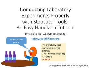
  • 88. A customer orders three bottles Three bottles please The probability that sour wine is served to him is 1-P(all bottles are good) = 1- 0.95^3 = 0.1426 VIN VIN VIN
  • 89. Comparisonwise vs Familywise error rate (restaurant owner) • The restaurant is worried not about the probability of each bottle being sour, but about the probability of accidentally serving sour wine to the customer who orders k bottles. The latter probability should be no larger than (say) 5%. YOU SERVED ME SOUR WINE I’M GONNA TWEET ABOUT IT
  • 90. Comparisonwise vs Familywise error rate (researcher) • We should be worried not about the comparisonwise Type I error rate, but about the familywise error rate – the probability of making at least one Type I error among the k=m(m-1)/2 tests. • Just repeating a t-test k times gives us a familywise error rate of 1-(1-α)^k if the tests are independent. e.g. α=0.05, k=10 ⇒ familywise error rate = 40%!
  • 91. Multiple comparison procedures [Carterette12][Nagata+97][Sakai18book] • Make sure that the familywise error rate is no more than α. • Stepwise methods: outcome of one hypothesis test determines what to do next • Single step methods: test all hypotheses at the same time – we discuss these only. - Bonferroni correction (considered obsolete) - Tukey’s Honestly Significant Difference (HSD) test - others (e.g. those available in pairwise.t.test)
  • 92. Bonferroni correction [Crawley15 ](pp.17-18) “The old fashioned approach was to use Bonferroni’s correction: in looking up a value for Student’s t, you divide your α value by the number of comparisons you have done. […] Bonferroni’s correction is very harsh and will often throw out the baby with the bathwater. […] The modern approach is […] to use the wonderfully named Tukey’s honestly significant differences” Or, equivalently, multiply each p-value by k
  • 93. Come back by 10:30!
  • 94. Tutorial Outline • Part I (9:00-10:00) - Preliminaries - Paired and two-sample t-tests, confidence intervals - One-way ANOVA and two-way ANOVA without replication - Familywise error rate [Coffee Break (10:00-10:30)] • Part II (10:30-12:00) - Tukey’s HSD test, simultaneous confidence intervals - Randomisation test and randomised Tukey HSD test - What’s wrong with statistical significance tests? - Effect sizes, statistical power - Topic set size design and power analysis - Summary: how to report your results IF YOU WANT MORE, PLEASE READ: Sakai, T.: Laboratory Experiments in Information Retrieval: Sample Sizes, Effect Sizes, and statistical power, to appear, Springer, 2018.
  • 95. • Instead of conducting a t-test k = m(m-1)/2 times, consider the maximum difference (best system – worst system) among the k differences. • The distribution that the max difference obeys is called a studentised range distribution. Its upper 100P% value is denoted by • We compare the k differences against the above distribution. By construction, if the maximum is not statistically significant, the other differences are not statistically significant either. Hence the familywise error rate can be controlled. How Tukey HSD works qtukey(P, m, φ, lower.tail=FALSE) in R
  • 96. Tukey HSD with equal group sizes (1) Data structure: same as one-way ANOVA with equal group sizes Tukey HSD can handle unequal group sizes as well. See [Sakai18book] sample mean for System i unpaired data
  • 97. Null hypothesis : the population means for systems i and i’ are equal Test statistic: Reject iff Tukey HSD with equal group sizes (2)
  • 98. R: Tukey HSD with equal group sizes The data.frame we made for one-way ANOVA Only the diff between Systems 1 and 3 statistically significant at α=0.05
  • 99. Tukey HSD with paired observations (1) Data structure: same as two-way ANOVA without replication sample mean for System i sample mean for Topic j paired data
  • 100. Null hypothesis : the population means for systems i and i’ are equal Test statistic: Reject iff Tukey HSD with paired observations (2)
  • 101. R: Tukey HSD with paired observations The data.frame we made for two-way ANOVA without replication The difference between Systems 1 and 3 and that between Systems 2 and 3 are statistically highly significant
  • 102. If you want a 95%CI for the diff between every system pair… • If you use the t-test-based MOE for every system pair, this approach has the same problem as repeating t-tests multiple times. • Use a Tukey-based MOE instead to construct a simultaneous CI – to capture all true means at the same time, not individually.
  • 103. Computing the MOE for simultaneous CIs From Tukey HSD with equal group sizes (unpaired data) From Tukey HSD with paired observations Apply the above MOE to each of the k differences
  • 104. R: Simultaneous 95%CI, equal group sizes (unpaired data) MOE = 0.081314 Upper limit = diff + MOELower limit = diff - MOE
  • 105. R: Simultaneous 95%CI, paired observations MOE = 0.033342 (CIs are narrower than the unpaired case) Upper limit = diff + MOELower limit = diff - MOE
  • 106. Tutorial Outline • Part I (9:00-10:00) - Preliminaries - Paired and two-sample t-tests, confidence intervals - One-way ANOVA and two-way ANOVA without replication - Familywise error rate [Coffee Break (10:00-10:30)] • Part II (10:30-12:00) - Tukey’s HSD test, simultaneous confidence intervals - Randomisation test and randomised Tukey HSD test - What’s wrong with statistical significance tests? - Effect sizes, statistical power - Topic set size design and power analysis - Summary: how to report your results IF YOU WANT MORE, PLEASE READ: Sakai, T.: Laboratory Experiments in Information Retrieval: Sample Sizes, Effect Sizes, and statistical power, to appear, Springer, 2018.
  • 107. Computer-based tests • Unlike classical significance tests, do not require assumptions about the underlying distribution • Bootstrap test [Sakai06SIGIR][Savoy97] – assumes the observed data are a random sample from the population. Samples with replacement from the observed data. • Randomisation test [Smucker+07] – no random sampling assumption. Permutes the observed data.
  • 108. Randomisation test for paired data (1) Suppose we have an nDCG matrix for two systems with n topics. Are these systems equally effective?
  • 109. Randomisation test for paired data (2) Suppose we have an nDCG matrix for two systems with n topics. Are these systems equally effective? Let’s assume there is a single hidden system. For each topic, it generates two nDCG scores. They are randomly assigned to the two systems.
  • 110. Randomisation test for paired data (3) If H0 is right, these alternative matrices (obtained by randomly permuting each row of U) could also have occurred
  • 111. Randomisation test for paired data (4) There are 2 possible matrices, but let’s just consider B of them (e.g. 10000 trials) n
  • 112. Randomisation test for paired data (5) How likely is the observed difference (or something even more extreme) under H0? → p-value
  • 113. Randomisation test for paired data - pseudocode The exact p-value changes slightly depending on B.
  • 114. Random-test in Discpower [Sakai14PROMISE] http://research.nii.ac.jp/ntcir/tools/discpower-en.html Contains a tool for conducting a randomisation test or randomised Tukey HSD test
  • 115. http://www.f.waseda.jp/tetsuya/20topics2runs.scorematrix Mean difference and p-value (compare with paired t-test) Paired randomisation test, B=5000 trials A 20x2 matrix, white-space-separated
  • 116. Randomised Tukey HSD test for paired data (1) Suppose we have an nDCG matrix for more than two systems with n topics. Are these systems equally effective?
  • 117. Suppose we have an nDCG matrix for more than two systems with n topics. Which system pairs are really different? Randomised Tukey HSD test for paired data (2) Let’s assume there is a single hidden system. For each topic, it generates m nDCG scores. They are randomly assigned to the m systems.
  • 118. If H0 is right, these alternative matrices (obtained by randomly permuting each row of U) could also have occurred Randomised Tukey HSD test for paired data (3)
  • 119. Randomised Tukey HSD test for paired data (4) There are (m!) possible matrices, but let’s just consider B of them (e.g. 10000 trials) n
  • 120. How likely are the observed differences given the null distribution of the maximum differences? → Tukey HSD p-value Randomised Tukey HSD test for paired data (5)
  • 121. Randomised Tukey HSD – pseudocode (adapted from [Carterette12]) The exact p-value changes slightly depending on B.
  • 122. http://www.f.waseda.jp/tetsuya/20topics3runs.scorematrix Randomised Tukey HSD test, B=5000 trials Compare the p-values with those of the Tukey HSD test with R (paired data) A 20x3 matrix, white-space-separated
  • 123. Tutorial Outline • Part I (9:00-10:00) - Preliminaries - Paired and two-sample t-tests, confidence intervals - One-way ANOVA and two-way ANOVA without replication - Familywise error rate [Coffee Break (10:00-10:30)] • Part II (10:30-12:00) - Tukey’s HSD test, simultaneous confidence intervals - Randomisation test and randomised Tukey HSD test - What’s wrong with statistical significance tests? - Effect sizes, statistical power - Topic set size design and power analysis - Summary: how to report your results IF YOU WANT MORE, PLEASE READ: Sakai, T.: Laboratory Experiments in Information Retrieval: Sample Sizes, Effect Sizes, and statistical power, to appear, Springer, 2018.
  • 124. [Bakan66] “The test of significance does not provide the information concerning psychological phenomena characteristically attributed to it; and a great deal of mischief has been associated with its use.”
  • 125. [Deming75] “Little advancement in the teaching of statistics is possible, and little hope for statistical methods to be useful in the frightful problems that face man today, until the literature and classroom be rid of terms so deadening to scientific enquiry as null hypothesis, population (in place of frame), true value, level of significance for comparison of treatments, representative sample.”
  • 126. [Loftus91] “Despite the stranglehold that hypothesis testing has on experimental psychology, I find it difficult to imagine a less insightful means of transiting from data to conclusions.”
  • 127. [Cohen94] (1) “And we, as teachers, consultants, authors, and otherwise perpetrators of quantitative methods, are responsible for the ritualization of null hypothesis significance testing (NHST; I resisted the temptation to call it statistical hypothesis inference testing) to the point of meaninglessness and beyond. I argue herein that NHST has not only failed to support the advances of psychology as a science but also has seriously impeded it.”
  • 128. [Cohen94] (2) “What’s wrong with NHST? Well, among many other things, it does not tell us what we want to know, and we so much want to know what we want to know that, out of desperation, we nevertheless believe that it does! What we want to know is “Given these data, what is the probability that H0 is true?” But as most of us know, what it tells us is “Given that H0 is true, what is the probability of these (or more extreme) data?”” p-value = Pr(D+| H) not Pr(H|D)! See also [Carterette15] [Sakai17SIGIR]
  • 129. [Rothman98] “When writing for Epidemiology, you can also enhance your prospects if you omit tests of statistical significance. Despite a wide spread belief that many journals require significance tests for publication, […] every worthwhile journal will accept papers that omit them entirely. In Epidemiology, we do not publish them at all. Not only do we eschew publishing claims of the presence or absence of statistical significance, we discourage the use of this type of thinking in the data analysis [….]”
  • 130. [Ziliak+08] “Statistical significance is surely not the only error in modern science, although it has been, as we will show, an exceptionally damaging one.” “Most important is to minimise Error of the Third Kind, “the error of undue inattention,” which is caused by trying to solve a scientific problem using statistical significance or insignificance only.”
  • 131. [Harlow+16] “The main opposition to NHST then and now is the tendency for researchers to narrowly focus on making a dichotomous decision to retain or reject a null hypothesis, which is usually not very informative to current or future research[…] Although there is still not a universally agreed upon set of practices regarding statistical inference, there does seem to be more consistency in agreeing on the need to move away from an exclusive focus on NHST […]”
  • 132. Statistical significance: Problem 1 Many misinterpret and/or misuse significance tests. American Statistical Association statement (March 2016): • P-values do not measure the probability that the studied hypothesis is true, or the probability that the data were produced by random chance alone. • A p-value, or statistical significance, does not measure the size of an effect or the importance of a result. p-value = Pr(D+|H) not Pr(H|D)!
  • 133. Statistical significance: Problem 2 Dichotomous thinking: statistically significant or not? (More important questions: - How much is the difference? - What does a difference of that magnitude mean to us?) p=0.049 ⇒ statistically significant at α=0.05 p=0.051 ⇒ NOT statistically significant at α=0.05 Reporting the exact p-value is more informative than saying “p<0.05” BUT THIS IS STILL NOT SUFFICIENT.
  • 134. Statistical significance: Problem 3 P-value = f(sample_size, effect_size) - A large effect size ⇒ a small p-value - A large sample size ⇒ a small p-value For example, consider: From the paired t-test Magnitude of the difference A large effect size (standardised mean difference) ⇒ a large t-value ⇒ a small p-value A large sample size (topic set size) ⇒ a large t-value ⇒ a small p-value Anything can be made statistically significant by making n large enough!
  • 135. Tutorial Outline • Part I (9:00-10:00) - Preliminaries - Paired and two-sample t-tests, confidence intervals - One-way ANOVA and two-way ANOVA without replication - Familywise error rate [Coffee Break (10:00-10:30)] • Part II (10:30-12:00) - Tukey’s HSD test, simultaneous confidence intervals - Randomisation test and randomised Tukey HSD test - What’s wrong with statistical significance tests? - Effect sizes, statistical power - Topic set size design and power analysis - Summary: how to report your results IF YOU WANT MORE, PLEASE READ: Sakai, T.: Laboratory Experiments in Information Retrieval: Sample Sizes, Effect Sizes, and statistical power, to appear, Springer, 2018.
  • 136. Effect size definition [Cohen88] “it is convenient to use the phrase “effect size” to mean “the degree to which the phenomenon is present in the population,” or “the degree to which the null hypothesis is false.” Whatever the manner of representation of a phenomenon in a particular research in the present treatment, the null hypothesis always means that the effect size is zero.”
  • 137. Effect size definition [Olejnik+03] “An effect-size measure is a standardized index and estimates a parameter that is independent of sample size and quantifies the magnitude of the difference between populations or the relationship between explanatory and response variable.”
  • 138. Effect size definition [Kelley+12] “Effect size is defined as a quantitative reflection of the magnitude of some phenomenon that is used for the purpose of addressing a question of interest.”
  • 139. Various effect sizes • Effect sizes for t-tests (and Tukey HSD): standardized mean differences (covered in this lecture) • Effect sizes for ANOVAs: contribution to the overall variance: see [Olejnik+03][Sakai18book] etc. for details • Other forms of effect sizes: see [Cohen88] etc.
  • 140. Paired t-test effect size Standardised mean difference (diff measured in standard deviation units) Note that sample size effect size Reporting dpaired along with the p-value is more informative than just reporting the p-value. But dpaired uses the standard deviation of the differences – works only with the paired t-test.
  • 141. Hedge’s g (1) Standardised mean difference for the two-sample case: Hedge’s g estimates the above: Common standard deviation Pooled variance
  • 142. Hedge’s g (2) From Student’s t-test, so, since , note that Reporting Hedge’s g along with the p-value is more informative than just reporting the p-value. See [Sakai18book] for bias correction. See [Sakai18book] for Cohen’s d
  • 143. Glass’s Δ (my favourite) • No homoscedasticity assumption! • Works for both paired and unpaired data! • A bias-corrected Δ: “How much is the difference, when measured in standard deviation units computed from the control group (i.e., baseline) data that we are familiar with?”
  • 144. Effect sizes for (randomised) Tukey HSD If homoscedasticity is assumed (as in classical Tukey HSD): If not, and if there is a common baseline, use Glass’ Δ by using the standard deviation of that baseline. Bottom line: report effect sizes as standardised mean differences, along with p-values. See “One-way ANOVA, equal group sizes (8)” See “Two-way ANOVA without replication (4)”
  • 145. Statistical power: ability to detect real differences Given α and an effect size that you are interested in (e.g. standardized mean difference >=0.2), increasing the sample size n improves statistical power (1-β). - An overpowered experiment: n larger than necessary - An underpowered experiment: n smaller than necessary (cannot detect real differences – a waste of research effort!) Can’t reject H0 Reject H0 H0 is true systems are equivalent Correct conclusion (1-α) Type I error α H0 is false systems are different Type II error β Correct conclusion (1-β)
  • 146. Tutorial Outline • Part I (9:00-10:00) - Preliminaries - Paired and two-sample t-tests, confidence intervals - One-way ANOVA and two-way ANOVA without replication - Familywise error rate [Coffee Break (10:00-10:30)] • Part II (10:30-12:00) - Tukey’s HSD test, simultaneous confidence intervals - Randomisation test and randomised Tukey HSD test - What’s wrong with statistical significance tests? - Effect sizes, statistical power - Topic set size design and power analysis - Summary: how to report your results IF YOU WANT MORE, PLEASE READ: Sakai, T.: Laboratory Experiments in Information Retrieval: Sample Sizes, Effect Sizes, and statistical power, to appear, Springer, 2018.
  • 148. On TREC topic set sizes [Voorhees09] “Fifty-topic sets are clearly too small to have confidence intervals in a conclusion when using a measure as unstable as P(10). Even for stable measures, researchers should remain skeptical of conclusions demonstrated on only a single test collection.” TREC 2007 Million Query track [Allan+08] had “sparsely-judged” 1,800 topics, but this was an exception…
  • 149. Deciding on the number of topics to create based on statistical requirements • Desired statistical power [Webber+08][Sakai16IRJ] • A cap on the confidence interval width for the mean difference [Sakai16IRJ] • Sakai’s Excel tools based on [Nagata03]: samplesizeTTEST2.xlsx (paired t-test power) samplesize2SAMPLET.xlsx (two-sample t-test power) samplesizeANOVA2.xlsx (one-way ANOVA power) samplesizeCI2.xlsx (paired data CI width) samplesize2SAMPLECI (two-sample CI width)
  • 150. Recommendations on topic set size design tools • If you’re interested in the statistical power of the paired t-test, two-sample t-test, or one-way ANOVA, use samplesizeANOVA2. • If you’re interested in the CI width of the mean difference for paired or two-sample data, use samplesize2SAMPLECI. • … unless you have an accurate estimate of the population variance of the score differences which the paired-data tools require. See “Paired t-test (1)” samplesizeTTEST2 samplesizeCI2
  • 151. samplesizeANOVA2 input α: Type I Error probability β: Type II Error probability, i.e., you want 100(1-β)% power (see below) m: number of systems to be compared in one-way ANOVA minD: minimum detectable range, i.e., whenever the true difference D between the best and the worst systems is minD or larger, you want to guarantee 100(1-β)% power : variance estimate for a particular evaluation measure (under the homoscedasticity assumption) μbest μworst D m system means
  • 152. samplesizeANOVA2: “alpha=.05, beta=.20” sheet (1) Enter values in the orange cells (α=5%, β=20%): m=10, minD=0.1, =0.1 To ensure 80% power (at α=5%) for one-way ANOVA with any m=10 systems with a minimum detectable range of 0.1 in terms of a measure whose variance is 0.1, we need n=312 topics. μbest μworst D>= 0.1 m system means
  • 153. samplesizeANOVA2: “alpha=.05, beta=.20” sheet (2) Enter values in the orange cells (α=5%, β=20%): m=2, minD=0.1, =0.1 To ensure 80% power (at α=5%) for one-way ANOVA with any m=2 systems with a minimum detectable difference of 0.1 in terms of a measure whose variance is 0.1, we need n=154 topics. μbest μworst D>= 0.1 Two system means
  • 154. samplesizeANOVA2: “alpha=.05, beta=.20” sheet (3) Since one-way ANOVA with m=2 systems is strictly equivalent to the two-sample t-test [Sakai18book], To ensure 80% power (at α=5%) for the two-sample t-test with a minimum detectable difference of 0.1 in terms of a measure whose variance is 0.1, we need n=154 topics. μbest μworst D>= 0.1 Two system meansThis n can also be regarded as a pessimistic estimate for the paired data case.
  • 155. samplesizeANOVA2: how does it work? (1) [Nagata03][Sakai16IRJ][Sakai18book] Remember what we do in one-way ANOVA: we reject H0 (all m means are equal) iff See “One-way ANOVA, equal group sizes (8)”
  • 156. samplesizeANOVA2: how does it work? (2) So, whether H0 is true or not, the probability of rejecting H0 is: If H0 is true, then F0 ~ F(φA, φE1) and the above = α Probability of incorrectly concluding that the system means are different
  • 157. samplesizeANOVA2: how does it work? (3) So, whether H0 is true or not, the probability of rejecting H0 is: If H0 is false, then F0 ~ F’(φA, φE1, λ) and the above = 1-β statistical power: probability of correctly concluding that the two system means are different A noncentral F distribution with a noncentrality parameter λ Accumulates squared system effects
  • 158. samplesizeANOVA2: how does it work? (4) If H0 is false, the power can be approximated as: where Let’s call it Formula P
  • 159. samplesizeANOVA2: how does it work? (5) Let’s ensure 100(1-β)% power whenever D >= minD (e.g., 0.1 in mean nDCG). To do this, we define: so that Δ >= minΔ holds. μbest μworst D m system means minΔ is the worst-case Δ for topic set sizes
  • 160. samplesizeANOVA2: how does it work? (6) • λ=nΔ so the worst-case topic set size n can be estimated very roughly as: where λ can be approximated using a linear function of φA for given (α, β). • Having thus obtained an n, check with Formula P to see if the desired power is really achieved. If not, n++. If the power is too high, n--, etc. • The excel tool does just that.
  • 161. samplesize2SAMPLECI input α: Type I Error probability for 100(1-α)% CIs δ: cap on the CI width for the difference between two systems (two-sample data). That is, you want the width of any CI to be δ or smaller. : variance estimate for a particular evaluation measure (under the homoscedasticity assumption) The n returned by samplesize2SAMPLECI can also be regarded as a pessimistic estimate for the paired data case. Difference in population means (a constant) : Width of this CI
  • 162. Enter values in the orange cells: α=5%, δ=0.1, =0.1 To ensure the CI width of any between-system difference to be 0.1 or smaller, we need n=309 topics. samplesize2SAMPLECI: “approximation” sheet
  • 163. samplesize2SAMPLECI: how does it work? (1) [Nagata03][Sakai16IRJ][Sakai18book] From “CIs for the difference in population means – unpaird data” we have: and the CI width is twice the MOE. We want 2MOE <= δ, but since Vp is a random variable, we use E(Vp) instead:
  • 164. samplesize2SAMPLECI: how does it work? (2) Consider a balanced design, n = n1 = n2 . Then the above can be approximated as: Let’s call it Inequality C
  • 165. samplesize2SAMPLECI: how does it work? (3) To obtain an initial estimate of n that satisfies the above, consider the CI for an ideal case where σ is known: cf. Inequality C Remember, the t- distribution is like a standard normal distribution with uncertainty
  • 166. samplesize2SAMPLECI: how does it work? (4) Hence • This gives us an optimistic estimate of n, so check with Inequality C. If the condition is not satisfied, n++, etc. • The excel tool does just that.
  • 167. Estimating the common variance If you have a topic-by-system score matrix or two from some pilot data, an unbiased estimator can be obtained as: Pooled estimate Estimate from one matrix See “Two-way ANOVA without replication (4)” A score matrix from test collection C
  • 168. Some real estimates based on TREC data (using VE1 rather than VE2) See “One-way ANOVA, equal group sizes (8)” Some measures are less stable ⇒ require larger topic set sizes under the same requirement
  • 169. Some topic set size design results [Sakai18book] The paired t-test tool does not return tight estimates due to my crude estimate (covariance not considered)
  • 170. So, to build a test collection… 1. Build a small data set first (or borrow one from a past task similar to your own). 2. Decide on a primary evaluation measure, and create a small topic-by-system score matrix with the small data set. 3. Compute as VE1 or VE2 and use a topic set size design tool to decide on n. 4. You can advertise your test collection as follows: “We created 70 topics, which, according to topic set size design with = 0.044, is more than sufficient for achieving 80% power with a (paired) t-test whenever the true difference in Mean nDCG@10 is 0.10 or larger.” See previous two slides
  • 171. Power analysis with R scripts [Sakai16SIGIR] (adapted from [Toyoda09]) • Given an adequately reported significance test result in a paper, - compute the effect size and the achieved power in that experiment. - propose a new sample size to achieve a desired power. Relies on the pwr library of R
  • 172. The five R power analysis scripts [Sakai16SIGIR] • future.sample.paired (for paired t-tests) • future.sample.unpairedt (for two-sample t-tests) • future.sample.1wayanova (for one-way ANOVAs) • future.sample.2waynorep (for two-way ANOVAs without replication) • future.sample.2wayanova2 (for two-way ANOVAs)
  • 173. future.sample.pairedt Basically just enter t0 and the actual sample size OUTPUT: - Effect size dpaired - Achieved power of the experiment - future sample size for achieving 80% power
  • 174. future.sample.pairedt: an actual example from a SIGIR paper A highly underpowered experiment. In future, use 244 topics, not 28, to achieve 80% power for this small effect (dpaired = 0.18). Only 15% power! Underpowered experiments can be a waste of research effort: there’s a high chance that you will miss a true difference! about 85%
  • 175. future.sample.2waynorep Basically just enter F0, the number of systems m and the actual sample size OUTPUT: - A partial effect size [Sakai18book] - Achieved power of the experiment - future sample size for achieving 80% power
  • 176. future.sample.2waynorep: an actual example from a SIGIR paper A highly underpowered experiment. In future, use 75 topics, not 17, to achieve 80% power for this small effect. Only 18% power! Underpowered experiments can be a waste of research effort: there’s a high chance that you will miss a true difference! about 82%
  • 180. Tutorial Outline • Part I (9:00-10:00) - Preliminaries - Paired and two-sample t-tests, confidence intervals - One-way ANOVA and two-way ANOVA without replication - Familywise error rate [Coffee Break (10:00-10:30)] • Part II (10:30-12:00) - Tukey’s HSD test, simultaneous confidence intervals - Randomisation test and randomised Tukey HSD test - What’s wrong with statistical significance tests? - Effect sizes, statistical power - Topic set size design and power analysis - Summary: how to report your results IF YOU WANT MORE, PLEASE READ: Sakai, T.: Laboratory Experiments in Information Retrieval: Sample Sizes, Effect Sizes, and statistical power, to appear, Springer, 2018.
  • 181. Reporting a paired t-test result (1) Clearly state the sample size within the table! Clearly indicate what the numbers are! Which evaluation measure? Are they mean values?
  • 182. Reporting a paired t-test result (2) “We conducted a paired t-test for the difference between our proposed system and the baseline in terms of mean nDCG over n=20 topics. The difference is not statistically significant (t(19) = 1.3101, p=0.2058, 95%CI[-0.0134, 0.0581]), with the effect size dpaired = t0/√n = 0.2929.” Provide as much information as possible for future researchers. There are several types of effect sizes. Clarify which one you are talking about.
  • 183. Reporting a two-sample t-test result (1) Clearly indicate what the numbers are! Which evaluation measure? Are they mean values? Clearly state the sample sizes within the table!
  • 184. Reporting a two-sample t-test result (2) “We conducted a Student’s t-test for the difference between the our proposed system (sample size n1 = 20) and the baseline (sample size n2 = 20) in terms of mean nDCG. The difference is not statistically significant (t(38) = 0.6338, p=0.53, 95%CI[-0.0491, 0.0938]), with Hedge’s g = 0.2004.” Note that If you used Welch’s t-test [Sakai16SIGIRshort], you consciously avoided the homoscedasticity assumption, so I recommend using Glass’ Δ, not Hedge’s d.
  • 185. Reporting a (randomised) Tukey HSD result (1)
  • 186. Reporting a (randomised) Tukey HSD result (2) “We conducted a randomised Tukey HSD test with B=5,000 trials to compare every system pair […] It can be observed that System 3 statistically significantly underperforms Systems 1 (p≒0.0000) and 2 (p=0.0024). Moreover, we computed an effect size ESE2 [Sakai18book] for each system pair. It can be observed that Systems 1 and 3 are almost two standard deviations apart from each other.” Also visualise each system’s performance using graphs with error bars, or boxplots! State clearly what the error bars represent (e.g., 95% CIs)!
  • 187. Summary • To design a test collection, use some pilot data to estimate the variance of a particular evaluation measure for sample size considerations. • To design an experiment, use a pilot or existing study for sample size considerations to ensure sufficient statistical power. Underpowered experiments can be a waste of research effort. • When reporting on statistical significance test results, report the sample sizes, test statistics, degrees of freedom, p-values (not the stars */**/***), and effect sizes! Despite what R outputs, it is wrong to decide on α AFTER looking at the results (e.g. “this difference is statistically significant at α=1% while that is significant at α=5%”)
  • 189. Thank you for staying until the end!
  • 190. References: A-B [Allan+08] Allan, J., Carterette, B., Aslam, J.A., Pavlu, V., Dachev, B., and Kanoulas, E.: Million Query Track 2007 Overview, Proceedings of TREC 2007, 2008. [Bakan66] Bakan, D.: The Test of Significance in Psychological Research, Psychological Bulletin, 66(6), pp.423-437, 1966.
  • 191. References: C-D [Carterette12] Carterette, B.: Multiple Testing in Statistical Analysis of Systems-based Information Retrieval Experiments, ACM TOIS 30(1), 2012. [Carterette15] Carterette, B.: Bayesian Inference for Information Retrieval Evaluation, ACM ICTIR 2015, pp.31-40, 2015. [Cohen88] Cohen, J.: Statistical Power Analysis for the Behavioral Sciences (Second Edition), Psychology Press, 1988. [Cohen94] Cohen, J.: The Earth is Round (p<.05), American Psychologist, 49(12), pp.997-1003, 1994. [Crawley15] Crawly, M.J.: Statistics: An Introduction Using R (Second Edition), Wiley, 2015. [Deming75] Deming, W.E., On Probability as a Basic for Action, American Statistician, 29(4), pp.146-152, 1975.
  • 192. References: G-H [Good05] Good, P.: Permutation, Parametric, and Bootstrap Tests of Hypothesis (Third Edition), Springer, 2005. [Harlow+16] Harlow, L.L., Mulaik, S.A., and Steiger, J.H.: What If There Were No Significance Tests? (Classic Edition), Routledge, 2016.
  • 193. References: K-L [Kelley+12] Kelly, K. and Preacher, K.J.: On Effect Size, Psychological Methods, 17(2), pp.137-152, 2012. [Loftus91] On the Tyranny of Hypothesis Testing in the Social Sciences, Contemporary Psychology, 36(2), pp.102-105, 1991.
  • 194. References: N-O [Nagata+97] Nagata, Y. and Yoshida, M.: Introduction to Multiple Comparison Procedures (in Japanese), Scientist press, 1997. [Nagata03] Nagata, Y.: How to Design the Sample Size (in Japanese), Asakura Shoten, 2003. [Olejnik+03] Olejnik, S. and Algina, J.: Generalized Eta and Omega Squared Statistics: Measures of Effect Size for Some Common Research Designs, Psychological Research, 8(4), pp.434-447, 2003.
  • 195. References: R [Robertson81] Robertson, S.E.: The Methodology of Information Retrieval Experiment, In Sparck Jones, K. (ed.): Information Retrieval Experiment, Chapter 1, Butterworths, 1981. [Robertson12] Robertson, S.E., Kanoulas, E.: On Per- topic Variance in IR Evaluation, ACM SIGIR 2012, pp.891-900, 2012. [Rothman98] Rothman, K.J.: Writing for Epidemiology, Epidemiology, 9(3), pp.333-337, 1998.
  • 196. References: S [Sakai06SIGIR] Sakai, T.: Evaluating Evaluation Metrics based on the Bootstrap, ACM SIGIR 2006, pp.525-532, 2006. [Sakai14PROMISE] Sakai, T.: Metrics, Statistics, Tests, PROMISE Winter School 2013: Bridging between Information Retrieval and Databases (LNCS 8173), Springer, 2014. [Sakai16IRJ] Topic Set Size Design, Information Retrieval, 19(3), pp.256-283, 2016. [Sakai16SIGIR] Sakai, T.: Statistical Significance, Power, and Sample Sizes: A Systematic Review of SIGIR and TOIS, 2006-2015, Proceedings of ACM SIGIR 2016, pp.5-14, 2016. [Sakai16SIGIRshort] Sakai, T.: Two Sample T-tests for IR Evaluation: Student or Welch?, Proceedings of ACM SIGIR 2016, pp.1045-1048, 2016. [Sakai17SIGIR] Sakai, T.: The Probability That Your Hypothesis Is Correct, Credible Intervals, and Effect Sizes for IR Evaluation, Proceedings of ACM SIGIR 2017, pp.25-34, 2017. [Sakai18book] Sakai, T.: Laboratory Experiments in Information Retrieval: Sample Sizes, Effect Sizes, and statistical power, to appear, Springer, 2018. [Salton+68] Salton, G. and Lesk, M.E.: Computer Evaluation of indexing and text processing, Journal of the ACM, 15, pp.8-36, 1968.
  • 197. References: S (continued) [Savoy97] Savoy, J.: Statistical Inference in Retrieval Effectiveness Evaluation, Information Processing and Management, 33(4), pp.495-512, 1997. [Smucker+07] Smucker, M.D., Allan, J. and Carterette, B.: A Comparison of Statistical Significance Tests for Information Retrieval Evaluation, CIKM 2007, pp.623-632, 2007. [SparckJones+75] Sparck Jones, K. and van Rijsbergen, C.J.: Report on the Need for and Provision of an ‘Ideal’ Information Retrieval Test Collection, Computer Laboratory, University of Cambridge, British Library Research and Development Report No.5266, 1975. [SparckJones81] Sparck Jones, K. (ed.): Information Retrieval Experiment, Butterworths, 1981. [SparckJones+97] Sparck Jones, K. and Willet, P.: Readings in Information Retrieval, Morgan Kaufmann, 1997.
  • 198. References: T [Toyoda09] Toyoda, H.: Introduction to Statistical Power Analysis: A Tutorial with R (in Japanese), Toyo Tosyo, 2009.
  • 199. References: V-W [VanRijsbergen79] Van Rijsbergen, C.J., Information Retrieval, Chapter 7, Butterworths, 1979. [Voorhees09] Voorhees, E.M.: Topic Set Size Redux, Proceedings of ACM SIGIR 2009, pp.806-807, 2009. [Webber+08] Webber, W., Moffat, A., and Zobel, J.: Statistical Power in Retrieval Experimentation, Proceedings of CIKM 2008, pp.571-580, 2008.
  • 200. References: Z [Ziliak+08] The Cult of Statistical Significance: How the Standard Error Costs Us Jobs, Justice, and Lives, The University of Michigan Press, 2008.