Global analysis of nonlinear dynamics

Chapter 2
Cell Mapping Techniques for Tuning
Dynamical Systems

´
Angela Castillo and Pedro J. Zufiria

Abstract In this chapter, to be dedicated in the 90th birthday of Professor C. S. Hsu,
several computational schemes are presented for the optimal tuning of the global
behavior of nonlinear dynamical systems. Specifically, the maximization of the size
of domains of attraction associated with invariants in parametrized dynamical
systems is addressed. Cell Mapping (CM) techniques are used to estimate the size
of the domains for different parameter values, and such size function is then
maximized via several optimization methods. First, a genetic algorithm is tested
whose performance shows to be good for determining global maxima at the expense
of high computational cost. Secondly, an iterative scheme based on a Stochastic
Approximation procedure (the Kiefer–Wolfowitz algorithm) is evaluated showing
acceptable performance at low cost. Finally, several schemes combining neural
network based estimations and model-based optimization procedures are addressed
with promising results. The performance of the methods is illustrated with some
applications including the well-known van der Pol equation with standard parame-
trization, and the tuning of a controller for saturated systems.

2.1 Introduction

Dynamical systems with tunable parameters are very common in many branches of
science and engineering. For instance, dynamic and control systems (Brockett and
Li 2003; Hu et al. 2002, 2005; Lewis 1987), robotic architectures (Arkin 1998; Fu
et al. 1987), and learning schemes (Mitchell 1997; Moore and Naidu 1983) are
processes whose behavior depends on the actual value of some characterizing
parameters. In other words, the properties of dynamical systems are parameter

´
A. Castillo (*) • P.J. Zufiria
´
Universidad Politecnica de Madrid, Madrid, Spain
e-mail: angela.castillo@upm.es; pedro.zufiria@upm.es

J.-Q. Sun and A.C.J. Luo (eds.), Global Analysis of Nonlinear Dynamics, 31
DOI 10.1007/978-1-4614-3128-2_2, # Springer Science+Business Media, LLC 2012

32 ´
A. Castillo and P.J. Zufiria

dependent. The number equilibria and their stability in parametrized dynamical
systems are widely studied in the framework of bifurcation theory (Seydel 1988).
The study and design of nonlinear dynamical systems based on global properties
(such as the size of attraction domains) cannot be easily addressed by standard
procedures. The study of attraction domains associated with asymptotically stable
system invariants is fundamental for global analysis. Some approaches for comput-
ing such domains of attraction can be seen in Flashner and Guttalu (1988), Guttalu
and Flashner (1988) and Xu et al. (1985). The tuning of these domains has great
applicability in the design of controllers (Hu et al. 2002), neural network models
(Cohen 1992), and the improvement of convergence in learning schemes (Moore
and Naidu 1983).
In this chapter, several computational schemes are considered for maximizing
the size of domains of attraction in certain parametrized dynamical systems. Cell
mapping (CM) techniques (Hsu 1987) are employed to estimate the size of those
regions, as presented in Castillo and Zufiria (2000, 2002, 2011). A genetic algo-
rithm, a Kiefer–Wolfowitz stochastic approximation procedure and several neural
network-based schemes are proposed as optimization methods for determining the
optimal parameter values.
Cell mapping-based schemes have also been employed for the design and
evaluation of optimal controllers (Hsu 1985; Hu et al. 1994a,b; Papa
´ ´ ´ ´
et al. 1997; Martınez-Marın and Zufiria 1999; Zufiria and Martınez-Marın 2003),
but only in cases where the cost functional can be approximated and optimized via
local procedures. In this chapter, a cell mapping-based global performance optimal
control is presented.
The rest of this chapter is organized as follows. The following section presents
the problem statement as well as the proposed procedure to address the problem.
Section 2.3 details some modifications performed on the cell mapping technique for
delineating and measuring the domains of attraction. The computational schemes
for finding optimal parameter values are detailed in Sect. 2.4. Simulation examples
are presented in Sect. 2.5. Concluding remarks appear in Sect. 2.6.

2.2 Problem Statement and Proposed Approach

We consider a family of dynamical systems defined by

_
x ¼ Fðx; aÞ; x 2 Rn ; a 2 I ; (2.1)

where I is a compact subset of ℝp. In addition, we consider a global performance index
J(a) ∈ ℝ, which naturally will also depend on the system parameter vector a ∈ I .

A parameter value a ∈ I is to be found such that the performance index is
maximized:

JðÞ ¼ maxfJðaÞ; a 2 I g:
a (2.2)

2 Cell Mapping Techniques for Tuning Dynamical Systems 33

It is well known that the existence of a is guaranteed, for instance, whenever J(a)
is a continuous function on the compact set I . Also, if J(a) is bounded (without
necessarily being continuous) in I , then the supremum sup{J(a), a ∈ I } exists.
Note that, although this supremum may not be reached for any value of a, numerical
optimization schemes may provide values of a such that J(a) is close enough to the
supremum. In the rest of the paper, without loss of generality, we will talk about
finding the maximum of J.
The performance index J may be difficult to compute since it is supposed to
gather global features. Hence, the use of numerical approximations becomes rele-
vant. First, one has to approximate (estimate) J(a) for any given value of a. Second,
J must be optimized, meaning that the maximum (or supremum) of {J(a), a ∈ I }
must be determined, using such approximated (estimated) values, without the
availability of any explicit algebraic expression for J. This condition is very restric-
tive and will determine the optimization algorithms that can be employed.
In this chapter, several algorithms are proposed which implement these two
steps as follows:
• J(a) is estimated making use of a cell mapping technique:

JðaÞ % J CM ðaÞ; a 2 I: (2.3)

This approximation is characterized in the following section.
• An approximation of max{JCM(a), a ∈ I } is computed using optimization
methods which are appropriate for dealing with the mentioned restriction
(non-availability of an algebraic expression). Precisely, Genetic Algorithms, a
Kiefer–Wolfowitz scheme, and some Neural Network-based techniques have
been employed.

2.2.1 Size of Domain of Attraction

The size of a domain of attraction is considered as the performance index J to be
maximized. Let us consider that 8a ∈ I , system (2.1) has an attractor at the
equilibrium point x∗, meaning that x∗ will have an associated attraction domain
D(x∗, a) which will depend on the parameter value a.
From a practical point of view, a working region H is defined, usually being an
n-dimensional rectangle ðH ¼ ½a1 ; b1 Š Â ½a2 ; b2 Š Â . . . Â ½an ; bn ŠÞ which contains
x∗ . Hence, the portion of the domain of attraction included in such region DH ¼
DðxÃ ; aÞ H is to be considered. (Note that if D(x∗, a) H then
DH ðxÃ ; aÞ ¼ DðxÃ ; aÞÞ.
A value a ∈ I of the parameter is to be found such that volðDH ðxÃ ; aÞÞ ¼

maxfvolðDH ðx Ã ; aÞÞ; a 2 I g. In this expression, vol(Á) is the mathematical function
which defines the volume of a region, so that the performance index can be defined as

JðaÞ ¼ volðDH ðxÃ ; aÞÞ; a 2 I : (2.4)

34 ´

As mentioned above, the existence of a in the compact set I is guaranteed if J(a) is
a continuous function.
The definition of JðaÞ ¼ volðDH ðxÃ ; aÞÞ ¼ lðDH ðxÃ ; aÞÞ is based on measure
theoretic concepts. Precisely, since D(x∗, a) is an open set and provided H is
compact, then DH ðxÃ ; aÞ is Lebesgue measurable. Nevertheless, we cannot guaran-
tee J(a) to be a continuous function, even if F ∈ C1(ℝn ÂI ). Fortunately, since H
is bounded, sup{J(a), a ∈ I } does exist.
The procedure proposed for the maximization of this specific performance index
J can be summarized as follows:
(a) First, the volume of D ðxÃ ; aÞ is estimated. This estimation can be performed
H
using the cell mapping technique (CM) (Hsu 1987), a computational method for
the global analysis of nonlinear dynamical systems. The use of CM requires the
selection of a rectangle in the state space region under consideration. This
rectangle does eventually define our working region H. Hence, the global analysis
will be restricted to such region. This rectangle is divided into cells, its comple-
mentary set being called sink cell. Based on that division of the state space, CM
can be applied to determine equilibria, limit cycles, and periodic solutions located
within the prescribed rectangle. Furthermore, if some attractor is found, CM
provides an approximation to its attraction domain in the rectangle (it will be
denoted DCM(x∗, a)), through the so-called cellular attraction domain.
Once CM has been applied, the computation of the volume of a cellular
domain is not difficult because it consists of cells, and cell dimensions are
known values. When referred to the problem considered here, CM can be
applied on H, and if x∗ is located, the volume of its associated cellular domain
will be considered as an estimation of the volume of DH ðxÃ ; aÞ.
Hence, the function to be maximized is the unknown

JðaÞ ¼ volðDH ðxÃ ; aÞÞ; (2.5)

and the function actually being optimized is its estimation

J CM ðaÞ ¼ volðDCM ðxÃ ; aÞÞ; (2.6)

which has no explicit algebraic expression.
(b) An optimization method to maximize JCM is required. For that purpose, an
algorithm able to maximize functions without explicit algebraic expression is
required. Three types of schemes are considered below.

2.2.2 Characterization of JCM

As mentioned above J(a) is estimated making use of the cell mapping technique:

JðaÞ % J CM ðaÞ; a 2 I: (2.7)


In this section, the statistical properties of JCM as an estimator of J are studied
in order to support the applicability of the optimization schemes employed in
this work.
The estimator JCM gathers several approximating steps:
• First, a partition of the state space into cells is defined, so that the domain is
approximated by a set of cells. This first step restricts the possible values of the
approximate domain size to be a multiple of the cell volume.
• In addition, the cell mapping carries out two additional approximations for the
(efficient) computation of the trajectories, which also depend on the cell size:
– The approximation due to the computation of trajectories only in a finite
interval.
– The approximation due to the use of numerical methods for computing such
trajectories.
We consider first the approximation due to the cell partitioning of the state space,
by neglecting errors in the computation of trajectories, since this error can be
analytically studied. Following the cell mapping definition, those cells in the
partition whose center point belongs to DH(x∗, a) will count as part of the approxi-
mation of DH(x∗, a). Such a set of cells, which is denoted as DP(x∗, a) (where P
stands for “Partition” into cells), can be seen as an approximation of the Lebesgue
measure of DH ðxÃ ; aÞ, which is defined by
X
lðDH ðxÃ ; aÞÞ¼ inf C volðci Þ; (2.8)
ci 2C

where C is a countable collection of cells whose union covers DH ðxÃ ; aÞ. Therefore,
we have that JðaÞ ¼ volðDH ðxÃ ; aÞÞ would be approximated by vol(DP(x∗, a)) if
the errors in the computation of trajectories were neglected.
Note that DP(x∗, a) depends on xo ¼ (a1, a2, . . ., an), the selected origin for H,
and on the cell size h. As mentioned above, a cell will belong to DP(x∗, a) if the
middle point of such a cell is included in DH ðxÃ ; aÞ. Based on a geometric
reasoning, one can expect that the error of the approximation comes from the
inclusion or exclusion of those cells ci containing points in the boundary of D
(x∗, a), that is, ci ∈ CB. These cells may or may not be included in DP(x∗, a),
depending on the fact that their center point belongs to DH ðxÃ ; aÞ. Note that xo can
be seen as a random variable. Hence, the inclusion or exclusion of vol(ci) in vol
(DP(x∗, a)) adds up an error to the estimator which can also be seen as a random
variable Eci . Although potentially Eci 2 ½ÀV; VŠ (V ¼ hn being the volume of a cell),
for small values of h and smooth domain boundaries (which can be approximated
by hyperplanes), one can expect Eci 2 ½À V ; V Š having a symmetric distribution
2 2
(which under some assumptions can be considered to be uniform). In any case,
2
EðEci Þ ¼ 0 and VarðEci Þ V .4
The total size of the cellular domain, vol(DP(x∗, a)), is computed as the sum of
the volumes of interior and boundary cells. The error associated with the total

36 ´

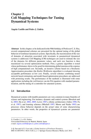
volume estimation, e, can be computed as the sum of the errors corresponding to the
boundary cells ci ∈ CB:
X
E¼ E ci : (2.9)
ci 2CB

It is important to note that Eci are not independent from each other, their joint
distribution strongly depending on the geometry of DH ðxÃ ; aÞ with respect to the
2
cell partitioning. In any case, the variance of e can be bounded VarðEÞ ð#CB Þ2 V , 4
ÀðnÀ1Þ
where #CB stands for the cardinality of CB. (Note that #CB ¼ Oðh Þ so that
VarðEÞ ¼ Oðh Þ and will tend to zero as h ! 0.)
2

Coming back to the cell mapping technique, besides the state space partition, it
computes an approximation of system trajectories in order to approximate
invariants and attraction domains. Such approximations include errors due to the
state space partition and also errors due to the computation of trajectories, as
explained above. Therefore, the cell mapping domain DCM(x∗, a) provides an
approximation of DH ðxÃ ; aÞ which in general will depend on xo and h as well as
on the numerical methods employed for the computation of trajectories. Hence, one
can also denote it as DCM(xo, h, p)(x∗, a), where p stands for the parameters
characterizing the numerical approximation of trajectories. Hence, one can charac-
terize the overall approximation of J(a) as follows

J CM ðaÞ ¼ J CMðxo ;h;pÞ ðxÃ ; aÞ ¼ volðDCMðxo ;h;pÞ ðxÃ ; aÞÞ ¼ JðaÞ þ x; (2.10)

where x is also a random variable which gathers e as well as numerical trajectory
computation errors.
Concerning the convergence of the approximation, one can prove that for the
simple cell mapping (SCM)

lim volðDCMðxo ;h;pÞ ðxÃ ; aÞÞ ¼ volðDH ðxÃ ; aÞÞ; (2.11)
h!0

that is, limh ! 0 JCM(xo, h, p)(x∗, a) ¼ J(a). This means that even if all the sources of
error are considered (due to the three types of approximations mentioned above),
convergence to the true value can be guaranteed as the cell size h tends to zero (see
Riaza and Zuﬁria 1999).
Note that in general JCM(a) has no explicit algebraic expression, and its distri-
bution cannot be characterized analytically. Also, the approximation error x (and
consequently, JCM(a)) will follow a distribution which depends on speciﬁc features
of the problem under analysis. In order to get some insight into the statistical
properties of JCM, some Monte Carlo simulations have been carried out. In particu-
lar, Figs. 2.1–2.3 show the results of the application of the Monte Carlo technique:
a rough estimation of the distribution of the random variable JCM(a) has been
obtained for three different problems.


Fig. 2.1 Estimation distribution for van der Pol with b ¼ 1

Fig. 2.2 Estimation distribution for van der Pol with b ¼ 5

38 ´

Fig. 2.3 Estimation distribution for saturated control system

2.3 Modifications to CM Implementation

Several remarks about the application and improvement of CM for estimating the
size of domains of attraction are presented in this section.
When CM is applied to analyze a dynamical system, some fake solutions can
appear. They are cellular invariants which do not correspond to invariants from the
original continuous system. These spurious invariants can show up due to either
slow dynamics or near to periodic solutions and equilibria. The effects of this type
of cellular solutions represent the main difficulty found in the application of CM to
our problem.
For instance, when approximating the domain of attraction of a single equilib-
rium point x∗ known to be the only invariant in a given region, CM might detect a
fixed cell where x∗ is located and another cellular invariant formed by k cells
around that fixed cell. This is clearly a fake cellular solution having its own cellular
attraction domain. A mistake will be made if only the cellular domain from the fixed
cell is taken as an approximation to the attraction domain of x∗. The appearance of
fake solutions might be avoided by changing some characteristics of the CM. If this
does not work, the two cellular domains can be joined providing the required
approximation.
This process of joining domains starts by distinguishing spurious solutions.
Then, one must associate their cellular domain of attraction with the corresponding


true invariant set. For doing so, the distance from a cellular invariant to each one of
the equilibria of the continuous system is computed first. If the minimum of those
distances is lower than a prescribed value, the invariant is considered spurious, its
cellular domain being associated with the nearest equilibrium point. If the mini-
mum distance is greater than the reference value, the invariant is not treated as a
fake solution.
In some cases the procedure introduced above may not avoid the effects due to
fake solutions. The success of this procedure is dependent on the type of dynamical
systems under consideration. For instance, in those systems which are known to
have a single attractor, all cells in the cellular attraction domains could be taken as
associated with the attractor.

2.4 Optimization Techniques

In this section, the main features of the different optimization schemes are outlined.

2.4.1 Genetic Algorithm

Genetic algorithms are search algorithms based on the dynamics of natural selec-
tion and natural genetics (Davis 1991; Goldberg 1989). They are mainly employed
for finding extreme points in functions where other methods do not work due to the
complexity or limitations in the search space. For instance, genetic algorithms are
appropriate in case that only raw function evaluations can be performed but no
additional information about the function (structure, derivatives, etc.) is available.
This is what happens in the type of problems treated in this chapter, where the only
available information is the value vol(DCM(x∗, a0)) for a given a0 ∈ I .
In general, a genetic algorithm starts from an initial population composed of
individuals (parameter values in our problem). Each individual is represented by
a code and evaluated by a fitness function (JCM in the problem treated here).
The algorithm develops processes of selection, crossover, mutation, and substitu-
tion. It tries to improve population fitness, generation by generation, and it finishes
when a certain percentage of identical individuals is reached, providing then the
best-found individual, which approximates the optimum we are pursuing. For more
information on genetic algorithms, see Davis (1991), Goldberg (1989) and
references therein.
The genetic algorithm used in the simulation examples of this chapter is a basic
particular case of the standard procedure: individuals are represented by binary
strings of 16 bits (in our case, an individual refers to a parameter value of the
dynamical system). Real coding could also be used, being especially suited for
multiparameter problems. Every generation is composed by 15 individuals; the
fitness function is taken as the function to be maximized (in our problem it is
JCM(a) ¼ vol(DCM(x∗, a)).

40 ´

The algorithm starts generating randomly 15 individuals which form the initial
population. Every bit value, 0 or 1, is selected with a probability of 1/2. Then, in the
selection process, individuals with a high fitness will have a high probability of
being selected. This probability is computed as a sum of two weighed terms. One of
them is the inverse of the number of individuals in a generation; the other one is the
normalized individual fitness (this is obtained dividing each fitness value by the
sum of the fitness values of all individuals in the actual generation).
Crossover follows the selection process. It constructs couples with adjoining
individuals in the list provided by the selection. Then, it interchanges pieces of
string between individuals in the same couple after a cross site has been randomly
selected. This affects only 60% of couples.
New individuals from crossover go through a mutation. This is accomplished by
a change (with a probability of 0. 3) in one of their bits chosen randomly.
Insertion of new individuals into the population is performed such that individuals
with a low fitness value will have a high probability of being replaced. Replacement
probabilities are obtained by subtracting the selection probabilities from 1.
After each insertion, the replacement probabilities are recalculated. The new
individual will have zero probability to be replaced again, and the rest of
probabilities will be normalized.
When crossover, mutation, and substitution have finished for all couples, the
process restarts for the new generation.
The algorithm finishes when 90% of individuals in a generation are identical.
Since the number of generations needed to fit such requirement can be too high, an
upper bound in the number of computed generations will be defined. This number is
chosen looking for a trade-off between obtaining a good approximation of the
optimal point and minimizing the computational time (i.e., calculating the smallest
number of fitness values). If the predefined maximum number of generations is
reached, the algorithm selects the individual showing the highest fitness value
during the whole process.

2.4.2 Kiefer–Wolfowitz Scheme

Loosely speaking, the Kiefer–Wolfowitz (K–W) algorithm is a stochastic version of
the well-known steepest descent (SD) optimization method for cases in which the
function to be maximized is not directly available. The SD algorithm is given by the
following dynamical systems:
• Discrete form

akþ1 ¼ ak þ Ek f a ðak Þ: (2.12)

• Continuous form

_
a ¼ f a ðaÞ; (2.13)


where f(Á) is the function to be maximized and fa(Á) is its derivative (one dimen-
sional case being considered).
SD can be applied if f(Á) and fa(Á) have known analytical expressions. In case
those functions were not available but noisy measurements of f(Á) could be
provided, then an option is estimating f(Á) and also its derivative. Incorporating
this idea to the SD method, the K–W algorithm appears, being defined by the
following difference equation:

akþ1 ¼ ak þ Ek ðf^ðak þ hÞ À f^ðak À hÞÞ=2h; (2.14)

where f^ðÁÞ represents a random variable which estimates f(Á). Note that in our
problem f is J and f^ is given by JCM; hence, the K–W scheme fits very well with
our data availability and associated computational costs.
Stochastic approximation theory assures that, under certain conditions on the
step size and the random variables characterizing the estimation procedure, this
algorithm converges to a local maximum of f(Á). This asseveration is based on the
fact that the equation given above follows in mean the differential equation (2.13),
the continuous version of the SD method. More details about K–W algorithm can be
found in Kushner and Yin (1997).

2.4.3 Neural Network-Based Schemes

One of the main uses of supervised neural networks (NN) is the approximation of
the explicit expression of a function f(Á) from which only raw sampling values are
known (Hassoun 1995).
Hence, the application of an NN to our problem will provide an analytical
approximation (let us say, g) of the function JCM(Á), so that its derivatives are easily
computed. The next step is to maximize the NN output value using an efficient
optimization method, for instance, the steepest descent algorithm or any other
traditional scheme, which can make use of the analytical expression of the function
to be maximized and its derivatives. Note that these derivatives can be computed
following a scheme that is similar to the back-propagation algorithm. One only
needs to take into account that:
P
• The derivative takes the form @g ¼ j dj wj .
@x
• dj can be computed recursively from dj + 1, satisfying the same relationship as in
the backpropagation algorithm.
• ds (output error) is equal to 1 (for the case of linear output).
Different schemes can be defined depending on the way that the training proce-
dure and optimization of the NN output are combined. For instance, the optimization
procedure can be carried out after an elaborated training, this procedure will be
labeled as NN(1) for comparative purposes. Besides that, the optimization procedure
can be alternated in the training process, being this scheme named NN(2).

42 ´

Alternatively, an online scheme can be implemented for getting initial
approximations of the maximum to be successively refined. Then, new data can
be computed in the neighborhood of this initial maximum estimate, in order to
refine such approximation. In addition, some function values that are far from the
initial estimate can also be incorporated, in order to avoid getting stuck in local
maxima. This procedure has been labeled as NN(3).

2.5 Simulation Examples

In this section, the effectiveness of the proposed techniques is tested on three
different dynamical systems. First, a dynamical system having a cubic term with
a complicated parameter dependency, second the well-known van der Pol equation
with standard parametrization, and finally the tuning of a controller with actuator
saturation (this problem depends on two parameters).

2.5.1 Example 1

In this example, the method is applied to a nonlinear system with a complicated
dependency on a parameter. The equations defining such system are

_
x1 ¼ ð1þ cos2 aÞx2 ;
_
x2 ¼ Àx2 þ ða2 À 10a þ 5Þðx1 À x1 3 Þ: (2.15)

The selected equilibrium point for the analysis is x∗ ¼ (0, 0). The rectangle
where CM is focused is H ¼ ½À4; 4Š Â ½À4; 4Š, and I ¼ [1, 9] is the set of param-
eter values where an optimum is looked for. Since (0, 0) is an attractor 8a ∈ I , we

can look for a 2 I = volðDðð0; 0Þ; aÞ HÞ ¼ maxfvolðDðð0; 0Þ; aÞ HÞ; a 2 I g.
As it has been explained in previous sections, we work with approximated values
for the function J(Á) ¼ vol(D(x∗, Á) H), the approximations being provided by
CM. Hence, JCM(Á) ¼ vol(DCM(x∗, Á)) will denote the function determined by the
CM approximations. In this example, the simple cell mapping (Hsu 1987) is used as
cellular method, classical fourth-order Runge–Kutta as numerical integration
method and the region H is split into 81 Â 81 cells.
The genetic algorithm chosen to maximize the mentioned function has the
structure and characteristics described in Sect. 2.4.1. In this case the maximum
number of generations will be fixed to 5, so that the number of fitness values to be
calculated is bounded by 15 Â 5 ¼ 75.


Fig. 2.4 Representation of function JCM(Á)

The algorithm has been run four times, providing as a result values of the
parameter a in the range [4. 6, 5. 1] with corresponding JCM values in
[13. 3, 14. 2]. It took the algorithm around 7 min for providing each estimation of

the a optimal value.
For the purpose of efﬁcient evaluation, JCM was computed for 1,000 values taken
randomly in I ¼ [1, 9] (this process took around 2 h and 30 min). The representa-
tion of those points can be seen in Fig. 2.4.
The results provided by the genetic algorithm are close to the real optimal value
of JCM in I ¼ [1, 9] (Fig. 2.4). This shows the good performance of the procedure
in this particular case. One of the cellular attraction domains computed in this
example can be seen in Fig. 2.5.
The simulation results for the different optimization methods are displayed in
the following table.

Time Solution
Genetic 420 s [4.6,5.1]
K–W 45 s 4.71
NN(1) 32 s 4.69
NN(2) 32 s 4.69
NN(3) 240 s 4.76

It is important to note that the highest computational cost is associated with the
function evaluation process. Taking this into account, each of the studied schemes
has speciﬁc features to be explained below. Hence, this table is only informative
and does not have precise comparative purposes.

44 ´

Fig. 2.5 Domain of attraction (Example 1)

As expected, the computational cost of the genetic algorithm applied to this
example is remarkably high, but it always provides an estimate of the global
optimum, although it may be not too accurate (ranging from 4. 6 to 5. 1).
Regarding K–W algorithm it has been checked that this method requires much
less computational time than the GA method, but it presents some risk of getting
stuck in a local maximum (20% of failure).
The computational requirements of the NN(1) are low when using a reduced set
of data, whereas a proper random selection of such data provides good results in
general. The whole computational cost (32 s) can be decomposed in 28 s for
obtaining data (evaluating the function), 3.8 s for network training and 0.02 s for
each SD iteration (very low cost). Once the network has been trained, the global
maximum can be easily determined by trying different initial conditions of the SD
method at very low cost.
The NN(2) method, which incorporates SD iterations during the NN training
process, has a similar computational cost to NN(1). The advantage of this method is
that it can incorporate some stopping criterion based on the sequence of maxima
provided by the SD method during the whole process. This means that the algorithm
may provide good results in early NN training stages without waiting for a
completely trained NN.
The NN(3) method being online oriented (such as GA and K–W) is computa-
tionally expensive due to the need of a higher number of function evaluations for
maximum reﬁnement purposes. This method also provides information concerning
the minimum number of data required for a good function approximation. This
information can be employed, for instance, in methods NN(1) and NN(2) (as
occurred in this simulation example).


Finally, it should be taken into account that all the NN methods provide an
analytical expression for the function approximation, an additional information not
obtained through the applications of the other alternative methods. Therefore, SD
can be applied in all NN-based methods a posteriori, using different initial
conditions, at low cost, thus avoiding the problem of local maxima.

2.5.2 Example 2

This example deals with the van der Pol equation and considers negative parameter
values. In that range the behavior is well known, having an unstable limit cycle,
with the origin as an attractor whose attraction domain happens to be the region
delimited by the limit cycle.
The equations of the system are

_
x1 ¼ x2 ;
(2.16)
_
x2 ¼ Àbð1 À x2 Þx2 À x1 :
1

The selected equilibrium point for the analysis is x∗ ¼ (0, 0). The rectangle
where CM is focused is H ¼ ½À8; 8Š Â ½À8; 8Š, and I ¼ [0. 1, 5] is the set of
parameter values where an optimum is searched for. Since (0, 0) is an attractor

8b 2 I , we can look for b 2 I = volðDðð0; 0Þ; bÞÞ ¼ maxfvolðDðð0; 0Þ; bÞÞ;

b 2 I g. In this example Dðð0; 0Þ; bÞ H, 8b 2 I , so the search process maximizes
the whole domain of attraction under consideration.
b
As in example 1, J CM ðÁÞ ¼ f ðÁÞ is characterized by using the SCM. Again, the
fourth order Runge–Kutta method is applied and H is divided into 161 Â161 cells.
The selected genetic algorithm follows again the structure and features men-
tioned in Sect. 2.4.1, having 5 as the maximum number of generations.
The algorithm has been run, spending around 20 min for providing each estimation

of the b optimal value. The adjoining cell mapping technique (ACM) (Guttalu and
Zufiria 1993; Zufiria and Guttalu 1993) was also tested being less time consuming but
providing worse estimates of the sizes of attraction domains. Looking for a compro-
mise between SCM and ACM, the use of the hybrid cell mapping technique seems to be
very promising (Riaza and Zufiria 1999). The SCM-based procedure obtained values
of the parameter b in the range [4. 97, 4. 99] with corresponding JCM values in
[28. 86, 28. 91]. Hence, it seems that the optimal value is reached at the upper extreme
of I . As a second part of the analysis in this example we searched for the parameter
value which minimizes the size of D((0, 0), Á) (i.e., maximizes the function vol
(H) À JCM(Á). The genetic algorithm provided values in [0. 58, 0. 69].
JCM has been computed for 500 values chosen uniformly in I ¼ [0. 1, 5]
(see Fig. 2.6). About 4 h and 30 min have been necessary for the whole computa-
tional process. It can be seen in Fig. 2.6 that the genetic algorithm provides fair
approximations to the minimizing parameter value in I ¼ [0. 1, 5]. Nevertheless,

46 ´

Fig. 2.6 Representation of function JCM(Á)

the location of such minimum could be improved via a further analysis focused in
the interval [0. 1, 1]. In this case, the obtained values are in [0. 17, 0. 23] with
function values in the range [12. 53, 12. 66]. These latest values are good
approximations of the minimum in I ¼ [0. 1, 5].
The results of the maximizing process and the minimizing (general and focused)
process are also represented in Fig. 2.6. The domain obtained for b ¼ 5,
corresponding to the maximum value, appears in Fig. 2.7.

2.5.3 Example 3: Control Tuning

This example considers the design of a control system with saturated actuators:

_
x ¼ Ax þ B Á satðFxÞ;
#
0 1 0
A¼ ; B¼ ; F ¼ ½f 1 ; f 2 Š: (2.17)
1 0 5

where sat(u) ¼ sign(u) Á min{1, |u|}. For ﬁxed feedback vector F ¼ ½À2; À1Š, this
system has x∗ ¼ (0, 0) as an asymptotically stable equilibrium point, and it has
been employed by several authors (see, for instance Hu et al. 2002, 2005) to
illustrate different schemes to estimate the domain of attraction via the use of
Lyapunov functions, being such estimates quite conservative. Here, the problem


Fig. 2.7 Domain of attraction for b ¼ 5 (Example 2)

of tuning feedback f1 and f2 components has been addressed in order to maximize
such domain of attraction.
The system can be deﬁned piecewise as follows:

_
x1 ðtÞ x2
¼ ; (2.18)
_
x2 ðtÞ x1 þ 5ðf 1 x1 þ f 2 x2 Þ

when j f1x1 + f2x2 j 1, and
#
_
x1 ðtÞ x2
¼ (2.19)
_
x2 ðtÞ x1 þ 5 signðf 1 x1 þ f 2 x2 Þ

elsewhere.
Note that the origin (0, 0) will always be an equilibrium point of the system.
Assuming f2 0, we get that for f1 À 0. 2 the origin is asymptotically
stable, and the system has two additional (unstable) equilibria at ( À 5, 0)
and (5, 0). Therefore, the analysis focuses on the region ðf 1 ; f 2 Þ 2 ðÀ1; À0:2Þ
ÂðÀ1; 0Þ.
When applying the different optimization approaches described in this chapter,
the results are quite sensitive to the initial conditions (seeds for the genetic scheme,
and initial conditions for Kiefer–Wolfowitz and NN schemes) since the domain
CM-estimate reaches a maximum in a parameter region including ðf 1 ; f 2 Þ 2
½À1:8; À0:6Š Â ½À2:0; À1:0Š as it can be seen at Fig. 2.8. In any case, the three

48 ´

Fig. 2.8 Representation of the cost function in Example 3

10
aprox_domain

5

0

−5

−10
−10 −5 0 5 10

Fig. 2.9 Domain of attraction for tuned feedback ðf 1 ; f 2 Þ ¼ ðÀ1:47; À1Þ (Example 3)

methods provide solutions within such region. Note that taking ðf 1 ; f 2 Þ ¼ ðÀ2; À1Þ
as in Hu et al. (2002, 2005) provides a domain CM-estimate smaller than when
choosing any pair of values in the mentioned optimal region.
Figure 2.9 shows the obtained domain of attraction for ðf 1 ; f 2 Þ ¼ ðÀ1:47; À1Þ
which is clearly larger than the previous existing estimates in the literature.


2.6 Concluding Remarks

Several computational methods to optimize domains of attraction in parametrized
dynamical systems have been introduced in this chapter. These methods employ
estimates provided by an adaptation of the cell mapping technique for the global
analysis of such systems. Three different schemes of optimization are used: genetic
algorithms, Kiefer–Wolfowitz algorithm, and Neural Network-based methods.
The good performance of the proposed procedures has been illustrated in three
particular examples, including the van der Pol nonlinear oscillator and the tuning of
a controller with actuator saturation.

Acknowledgments This work has been partially supported by project MTM2007-62064 of the
Plan Nacional de I+D+i, MEyC, Spain, project MTM2010-15102 of Ministerio de Ciencia
´
e Innovacion, Spain, and by projects Q09 0930-182 and Q10 0930-144 ofthe Universidad
´
Politecnica de Madrid (UPM), Spain.

References

Arkin RC (1998) Behavior-based robotics. The MIT Press, Cambridge
Brockett RW, Li H (2003) A light weight rotary double pendulum: Maximizing the domain of
attraction. In: Proceedings of 42 IEEE CDC, Maui, Hawaii USA, pp 3299–3304
´
Castillo A, Zufiria PJ (2000) A computational method for maximizing domains of attraction in
dynamical systems. Eighth international conference on information processing and manage-
ment of uncertainty in knowledge-based systems (IPMU2000), pp 165–171, Madrid
´
Castillo A, Zufiria PJ (2002) Hybrid schemes for parameter tuning of nonlinear dynamical
systems. First international NAISO congress on neuro fuzzy technologies, 100027-01-AC-
073. ICSC NAISO Academic Press Canada/The Netherlands, pp 74–80
´
Castillo A, Zufiria PJ (2011) Computational schemes for optimizing domains of attraction in
dynamical systems. In: Proceedings of the ASME 2011 international design engineering
technical conferences computers and information in engineering conference, DETC2011-
48158, 10 pp, Washington, DC
Cohen MA (1992) The construction of arbitrary stable dynamics in nonlinear neural networks.
Neural Network 5:83–103
Davis L (1991) Handbook of genetic algorithms. VNR Computer Library, New York
Flashner H, Guttalu RS (1988) A computational approach for studying domains of attraction for
non-linear systems. Int J Non-Linear Mech 23(4):279–295
´
Fu KS, Gonzalez RC, Lee CSG (1987) Robotics: Control, sensing, vision and intelligence.
McGraw-Hill Book Company, New York
Goldberg DE (1989) Genetic algorithms in search, optimization and machine learning. Addison-
Wesley Publishing company, Boston
Guttalu RS, Flashner H (1988) A numerical method for computing domains of attraction for
dynamical systems. Int J Numer Meth Eng 26:875–890
Guttalu RS, Zufiria PJ (1993) The adjoining cell mapping and its recursive unraveling, Part II:
Application to selected problems. Nonlinear Dynam 4:309–336
Hassoun MH (1995) Fundamentals of artificial neural networks. MIR Press, Cambridge
Hsu CS (1985) A discrete method of optimal control based upon the cell state space concept.
J Optim Theor Appl 46:547–569
Hsu CS (1987) Cell-to-cell mapping. Springer, New York

50 ´

Hu T, Goebel R, Teel AR, Lin Z (2005) Conjugate Lyapunov functions for saturated linear
systems. Automatica 41:1949–1956
Hu T, Lin Z, Chen BM (2002) An analysis and design method for linear systems subject to actuator
saturation and disturbance. Automatica 38:351–359
Hu HT, Tai HM, Shenoi S (1994a) Fuzzy controller design using cell mappings and genetic
algorithms. In: Wang PP (ed) Advances in fuzzy theory and technology, vol 2. Bookwrights,
Durham, NC, pp 243–264
Hu HT, Tai HM, Shenoi S (1994b) Incorporating cell map information in fuzzy controller design.
In: Proceedings of the third IEEE international conference on fuzzy systems, pp 394–399
Kushner HM, Yin GG (1997) Stochastic approximation algorithms and applications. Springer,
New York
Lewis FL (1987) Optimal control. Wiley, New York
´ ´
Martınez-Marın T, Zufiria PJ (1999) Optimal control of nonlinear systems through hybrid Cell-
Mapping/Artificial Neural-Networks techniques. Int J Adapt Contr Signal Process 13:307–319
Mitchell TM (1997) Machine learning. WCB/McGraw-Hill, Boston
Moore KL, Naidu DS (1983) Maximal domains of attraction in a Hopfield neural network with
learning. In: Proceedings of American control conference, pp 2894–2896
Papa M, Tai HM, Shenoi S (1997) Cell mapping for controller design and evaluation. IEEE Contr
Syst Mag 17(2): 52–65
Riaza R, Zufiria PJ (1999) Adaptive cellular integration of linearly implicit differential equations.
J Comput Appl Math 111:305–317
Seydel R (1988) From equilibrium to chaos: Practical bifurcation and stability analysis. Elsevier,
New York
Xu J, Guttalu RS, Hsu CS (1985) Domains of attraction for multiple limit cycles of coupled van der
Pol equations by simple cell mapping. Int J Non-Linear Mech 20(5/6):507–517
Zufiria PJ, Guttalu RS (1993) The adjoining cell mapping and its recursive unraveling, Part I:
Description of adaptive and recursive algorithms. Nonlinear Dynam 4:207–226
´ ´
Zufiria PJ, Martınez-Marın T (2003) Improved optimal control methods based upon the adjoining
cell mapping technique. J Optim Theor Appl 118(3):657–680

http://www.springer.com/978-1-4614-3127-5

Global analysis of nonlinear dynamics

Recomendados

Recomendados

Mais conteúdo relacionado

Mais procurados

Mais procurados (19)

Destaque

Destaque (19)

Semelhante a Global analysis of nonlinear dynamics

Semelhante a Global analysis of nonlinear dynamics (20)

Mais de Springer

Mais de Springer (20)

Último

Último (20)

Global analysis of nonlinear dynamics