2019 SWCS International Annual Conference July 28-31, 2019 Pittsburgh, Pennsylvania

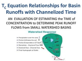
1. AN EVALUATION OF ESTIMATING the TIME of
CONCENTRATION to DETERMINE PEAK RUNOFF
FLOWS from SMALL WATERSHED BASINS
TC Equation Relationships for Basin
Runoffs with Channelized Time

2.  Surface Conditions / Soil Type
 Watershed Size / Length of Runoff
 Basin Slope / Rainfall Depth
 Four Types of Surface Runoff Coefficients are
Evaluated & Compared to Impervious Surface.
 NRCS’s Segmental Equations are Calculated &
Graphically Displayed by Watershed Attributes.
 Three Different Tc Empirical Equations are
Compared to NRCS’s Segmental Calculations.
This Presentation Offers Insight to Tc Calculations &
Tc Analogies in Small Watersheds for the Following:
Factors Affecting Stormwater Runoff:

3. Taken from Wanielista, M., R. Kersten, and R. Eaglin,
Hydrology: Water Quantity and Quality Control, p. 184
SCS Method
Time of Concentration’s Definition
Time of Concentration tc:
Time required for water
to travel from the most
hydraulically remote
point in the basin to the
basin outlet.
This time is determined by
drainage characteristics such as
surface density, slope, channel
roughness, and soil infiltration.
Many empirical equations have
been developed through
watershed research.

4. Velocity Equations Used in
NRCS Segmental Method
• Sheet Flow – Overland Flow
• Shallow Flow (Rills and Gullies)
• Open Channel/Pipe Flow (Conveyance)

5. Sheet Flow
TR-55 Sheet Flow—The sheet flow time computed for each area of
sheet flow that requires the following input data:
Hydraulic Length—Defined flow length for the sheet flow.
Manning's n—Manning's roughness value of the sheet flow.
Slope— The defined slope of the sheet flow/catchment.
Precipitation
Infiltration
A basin unit flow expressed by
an implicit channelized flow
(Not basin surface area flow)
Manning’s Kinematic
Wave Eq.

7. Sheet Flow Limitations
National Engineering Handbook
Kibler and Aron (1982) and others indicated the maximum sheet
flow length is less than 100 feet. To support the sheet flow limit of
100 feet, Merkel (2001) reviewed a number of technical papers on
sheet flow. McCuen and Spiess (1995) indicated larger sheet flow
length variables lead to less accurate designs, and proposed a
limitation with equation (15–8) shown below be considered:
Eq. 15-8 𝒍 =
𝟏𝟎𝟎 𝑺
𝒏
where:
n = Manning’s roughness coefficient
l = limiting length of flow (ft)
S = slope (ft/ft)

8. What are ‘n’ Sheet Flow Relationships
to Other Surface Runoff Values?
Percent
Impervious
Manning’s Low ‘n’
Sheet Flow Values
Manning’s High ‘n’
Sheet Flow Values
Manning’s Average ‘n’
Sheet Flow Values
1% 0.700 0.800 0.750
0.450 0.550 0.500
30% 0.300 0.480 0.390
0.160 0.420 0.290
0.100 0.200 0.150
0.022 0.033 0.028
99% 0.011 0.015 0.013

9. Sheet Flow ‘n’ Coefficient Interpolated to
Percent Impervious Surface
Percent
Impervious
Exponential
‘n’Values
Linear ‘n’
Values
Polynomial
‘n’Values
Average ‘n’ Sheet
Flow Values
1% 0.750 0.750 0.750 0.750
10% 0.650 0.623 0.625 0.633
20% 0.424 0.551 0.501 0.492
30% 0.276 0.480 0.390 0.382
40% 0.180 0.408 0.293 0.294
50% 0.117 0.337 0.211 0.222
60% 0.076 0.265 0.143 0.162
70% 0.050 0.194 0.089 0.111
80% 0.032 0.122 0.049 0.068
90% 0.021 0.051 0.024 0.032
99% 0.013 0.013 0.013 0.013

10. Shallow Concentrated Flow
V
L
t 
NRCS definition of shallow flow is 1 inch to 6 inches deep
Chapter 15
Part 630
of National
Engineering
Handbook
Channelized Flow Time

11. Shallow Flow Equations from NEH, May 2010

12. Shallow Flow Velocity Equations for
0.25 ft. of Depth and Manning's “n”
Mannings
“n” Value
Depth of
Flow (ft.)
Velocity Equations (ft./s)
0.200 0.25 V = 2.949(s)0.5
0.160 0.25 V = 3.686(s)0.5
0.130 0.25 V = 4.536(s)0.5
0.110 0.25 V = 5.361(s)0.5
0.086 0.25 V = 6.857(s)0.5
0.067 0.25 V = 8.802(s)0.5
0.052 0.25 V = 11.341(s)0.5
0.039 0.25 V = 15.121(s)0.5
0.029 0.25 V = 20.335(s)0.5
0.022 0.25 V = 26.805(s)0.5
0.013 0.25 V = 45.363(s)0.5

13. Open Channel Flow Equation
2/13/249.1
SR
n
V 
Tc conveyance flow = Length / Velocity
Manning’s
Equation
Hydraulic Radius Can Equal Flow Depth in
Manning’s Eq. for Small-Wide Channels
NRCS’s considers 6 in. or deeper to be channel flow
An initial 8 in. depth is used to initiate channel flows
& increased to 16 in. depth for an average depth of 1 ft.
Conveyance Flow
for Uniform
Geometry

14. Manning’s ‘n’ Channel Coefficients
From USACE, January 2010, HEC-RAS River Analysis System, Hydraulic Reference Manual, Version 4.1.

15. Velocity Equations with an 8 to 16 Inch
Flow Depth for a Channel “n” Value
Mannings
“n” Value
Initial Depth
of Flow (ft.)
Velocity Equations (ft./s)
Ending Depth
of Flow (ft.)
Velocity Equations
(ft./s)
0.140 0.67 V = 8.127(s)0.5 1.35 V = 13.157(s)0.5
0.120 0.67 V = 9.482(s)0.5 1.35 V = 15.349(s)0.5
0.100 0.67 V = 11.378(s)0.5 1.35 V = 18.419(s)0.5
0.085 0.67 V = 13.386(s)0.5 1.35 V = 21.670(s)0.5
0.074 0.67 V = 15.376(s)0.5 1.35 V = 24.891(s)0.5
0.057 0.67 V = 19.962(s)0.5 1.35 V = 32.314(s)0.5
0.042 0.67 V = 27.091(s)0.5 1.35 V = 43.855(s)0.5
0.034 0.67 V = 33.465(s)0.5 1.35 V = 54.174(s)0.5
0.027 0.67 V = 42.141(s)0.5 1.35 V = 68.219(s)0.5
0.021 0.67 V = 54.181(s)0.5 1.35 V = 87.711(s)0.5
0.012 0.67 V = 94.817(s)0.5 1.35 V = 153.494(s)0.5

16. Total Hydraulic Time Calculations
(TR55, Velocity, or SCS Method)
Sheet Flow Tt = 0.007(nL)0.8/(P2
0.5S0.4)
Shallow Concentrated Flow Tt = L /3600V
Open Channel Flow Tt= (L*n) /(1.49R0.67S 0.5)
(Manning’s Equation)
Where Hydraulic Radius = conveyance flow depth then:
Manning’s equation becomes Tt = L/3600V
Total Watershed Time of Concentration
tc=STt
L= ft., Tt = hr., S= % slope, R= ft., P= in.(2yr.24hr.) , V= ft./sec.

17. Visualizing Tc with Manning’s ‘n’, McCuren
& Spiess Limits, & NRCS Velocity Equations
• Sheet flow lengths are 90-110 ft. for 2 & 10% slopes
respectively at a full impervious surface then
reduced by 10% for each 10% drop in impervious
area towards a no impervious woods with 30-40 ft.
flow lengths for a 2 & 10% slope respectively.
• Shallow concentrated flow lengths are 400-500 ft.
for 2 & 10% slopes respectively at a full impervious
surface then reduced by 10% for each 10% drop in
impervious area towards a no impervious woods
with 140-175 ft. flow lengths for a 2 & 10% slope.

18. Visualizing TC with Manning’s ‘n’, McCuren
& Spiess Limits, & the Velocity Equations
• The remaining flow path length is considered
channel flow with a comparable Manning’s ‘n’
coefficient to the sheet flow and shallow flow.
• The equations consider flow, path geometry, slope,
and surface conditions homogenous.
• NEH has noted by Folmar & Miller (2008) that it was
discovered the velocity method can underestimate
time of concentration for larger watersheds.
The Following Plot is TC Velocity Eq. Boundary:

19. Tc Pervious & Impervious Boundaries
for 1% & 12% Basin slopes Respectively

20. Implicit assumptions from the graph
• The very high impervious surfaces basins are
defined by the lower graph line and high pervious
surfaces basins are defined by upper graph line.
• Most hydrographs are defined by the area between
the upper & lower graph lines. Typical designs use
Tc’s between the two lines to create hydrographs.
• The following interpolations for relationships of %
impervious, CN, C, & “n” values will help establish
these commonly used Tc values in a watershed.

21. NRCS’s ‘CN’ Values for Soil Groups

22. Percent Impervious Surface to the
Soil Group’s Average ‘CN’ Value
Percent
Impervious
Soil
Group A
Soil
Group B
Soil
Group C
Soil
Group D
Average ‘CN’
Value for All
1% 30 55 70 77 58.00
12% 46 65 77 82 67.50
20% 51 68 79 84 70.50
25% 54 70 80 85 72.25
30% 57 72 81 86 74.00
38% 61 75 83 87 76.50
65% 77 85 90 92 86.00
72% 81 88 91 93 88.25
85% 89 92 94 95 92.50
99% 98 98 98 98 98.00

23. Rational ‘C’ Coefficient with Soil Types

24. Percent Impervious Surface to the
Soil Group’s Average ‘C’ Value
Percent
Impervious
Soil
Group A
Soil
Group B
Soil
Group C
Soil
Group D
Average ‘C’
Value for All
1% 0.095 0.125 0.145 0.180 0.137
12% 0.208 0.235 0.277 0.320 0.260
20% 0.225 0.245 0.285 0.320 0.269
25% 0.245 0.275 0.310 0.340 0.293
30% 0.275 0.305 0.335 0.360 0.319
38% 0.300 0.330 0.355 0.380 0.341
65% 0.370 0.400 0.420 0.450 0.410
72% 0.765 0.770 0.775 0.775 0.771
85% 0.795 0.805 0.805 0.805 0.803
99% 0.910 0.910 0.910 0.910 0.910

25. 10% Impervious Surface Increments
Normalized to ‘CN’ & ‘C’ Coefficients
These Values are Plotted in the Following Graphs:
Percent
Impervious
Average ‘n’ Sheet
Flow Coefficients
Calculated Average
‘CN’ Value from %
Calculated Average
‘C’ Value from %
1% 0.750 58.0 0.14
10% 0.655 63.5 0.19
20% 0.511 68.1 0.25
30% 0.395 72.6 0.31
40% 0.302 76.8 0.38
50% 0.225 80.8 0.46
60% 0.161 84.6 0.54
70% 0.106 88.3 0.63
80% 0.060 91.7 0.72
90% 0.021 94.9 0.82
99% 0.013 98.0 0.91

26. Flow Path vs. TC for 2% slope path

27. Flow Path vs. TC for 5% slope path

28. Flow Path vs. Tc for 10% slope path

29. Kirpich Tc Equation
Tc=
𝟎.𝟎𝟎𝟕𝟖 𝑳 𝒄
𝟎.𝟕𝟕
𝑺 𝒄
𝟎.𝟑𝟖𝟓
A Tc equation modeled from channelized basins
• Tc = minutes, Lc = flow path length (ft.)
Sc = flow path slope in (ft./ft.)
• Kirpich is an accepted method in estimating Tc on small basins
(1 - 112 acres). It was developed from 7 rural watersheds with
basin slopes (3 to 10%) for an assumed bare soil flow paths.
• The slope Sc is the elevation difference between the most remote
point to the outlet divided by the flow path length Lc.

30. Comparisons of Kirpich Equation
Factors to other Runoff Coefficients
Ground Cover Kirpich Adjustment Factor, ‘k’
(Chow, 1988; Chin, 2000)
General overland flow and natural grass channels 2.0
Overland flow on bare soil or roadside ditches 1.0
Overland flow on concrete or asphalt surfaces 0.4
Flow in concrete channels 0.2
Ground Cover
Kirpich
Adjustment
Factor, ‘k’
Estimated
‘C’ Value
from Cover
Estimated
‘CN’ Value
from Cover
Estimated
Percent (%)
Impervious
Natural Grass 2.0 .30 72 29
Bare Soil or
Roadside ditch
1.0 .49 82 54
Flow on concrete /
asphalt surfaces
0.4 .91 98 99

31. Extrapolation of Kirpich’s ‘k’ Factor
Percent
Impervious
Linear ‘k’
Values
Exponential
‘k’ Values
Polynomial
‘k’ Values
Average ‘k’ Kirpich
Adjustment factor
1% 2.43 3.59 3.69 3.24
12% 2.19 2.80 2.95 2.65
20% 2.02 2.33 2.48 2.28
25% 1.91 2.08 2.20 2.07
30% 1.80 1.86 1.95 1.87
38% 1.63 1.55 1.59 1.59
65% 1.04 0.84 0.71 0.86
72% 0.89 0.72 0.57 0.73
85% 0.60 0.53 0.42 0.52
99% 0.30 0.39 0.40 0.36

32. Extrapolated ‘k’ Factor for Maximum
Projected 2.9 ‘k’ & minimum 0.35 ‘k’
Basin’s
Percent
Impervious
Kirpich ‘k’
Adjustment
factor
1% 2.93
10% 2.58
20% 2.21
30% 1.88
40% 1.57
50% 1.30
60% 1.04
70% 0.82
80% 0.63
90% 0.46
99% 0.34

33. Average ‘CN’, ‘C’, ‘k’, & ‘n’ Coefficients
Normalized to 10% Impervious Surface
Percent
Impervious
Calculated ‘CN’
Values from %
Calculated ‘C’
Values from %
Kirpich ‘k’
Values from %
‘n’ Sheet Flow
Coefficients
1% 58.0 0.14 2.93 0.750
10% 63.5 0.19 2.58 0.655
20% 68.1 0.25 2.21 0.511
30% 72.6 0.31 1.88 0.395
40% 76.8 0.38 1.57 0.302
50% 80.8 0.46 1.30 0.225
60% 84.6 0.54 1.04 0.161
70% 88.3 0.63 0.82 0.106
80% 91.7 0.72 0.63 0.060
90% 94.9 0.82 0.46 0.021
99% 98.0 0.91 0.34 0.013

34. Kirpich & Velocity Eq. Tc’s Compared

35. Kirpich & Velocity Eq. Tc’s Compared

36. Kirpich & Velocity Eq. Tc’s Compared

37. NRCS’s LAG Equation
Tlag
=
𝑳 𝒄
𝟎.𝟖 𝟏𝟎𝟎𝟎
𝑪𝑵
−𝟗
𝟎.𝟕
𝟏𝟗𝟎𝟎 𝒀 𝒄
𝟎.𝟓
Tc = 𝟔𝟎
𝑻𝒍𝒂𝒈
𝟎.𝟔
𝐈𝐅 𝐂𝐅
A TC equation formed with the basin’s surface data
• Tlag
=Lagtime(hrs.), Lc
=flowpathlength(ft.)
• Yc = average watershed slope number percent (%)
• Tc
=TimeofConcentration(minutes) IF&CF=FHWA Adjust.Factors
NRCS lag method was developed by Mockus in 1961 for many conditions
from heavy forest, meadows, and paved areas less than 2000 acres.
Referenced by NRCS as a TC.

38. NRCS Lag & Velocity Tc’s Compared

39. FHWA (HEC19) Adjustment Factors for NRCS Lag
Eq. on imperviousness & channel improvements
𝐌 = 𝟏 − 𝐩 −𝟔. 𝟖 𝟏𝟎 −𝟑
+ 𝟑. 𝟒 𝟏𝟎 −𝟒
𝑪𝑵 − 𝟒. 𝟑 𝟏𝟎 −𝟕
𝑪𝑵 𝟐
𝟐. 𝟐 𝟏𝟎 −𝟖
𝑪𝑵 𝟑
𝐌 = NRCS’s adjustment factors on Lag Eq. for percent imperviousness and channel improvements
𝐩 = the percent imperviousness or percent of main channels that are hydraulically improved
beyond natural conditions.

40. Lag Imp. & Channel Factors vs. Velocity

41. Lag Imp. & Channel Factors vs. Velocity

42. Lag Imp. & Channel Factors vs. Velocity

43. FAA’s TC Equation
Tc = 𝟏. 𝟖 (𝟏. 𝟏 − 𝑪)
𝑳 𝒄
𝟎.𝟓
𝑺 𝒄
𝟎.𝟑𝟑
A TC equation formed with basin’s surface data
Tc = minutes, Lc = flow path length (ft.)
Sc = flow path slope in (% full number)
C= Rational Runoff Coefficient
• Developed from airfield drainage with data assembled by USACE.
It is frequently used on urban watersheds.
• This equation was developed in an environment of primarily
sheet & shallow flow, low slopes, higher impervious surfaces, and
on small drainage basins.

44. FAA TC vs. Velocity TC’s Compared
No Channelization Factor

45. Small Watershed Runoff Response
• TC comparison graphs between the velocity equations and channelized empirical
equations convey a systematic intersect for each related surface coefficient.
• Empirical equations provide a lower TC in short flow paths while velocity
equations for a same flow path exhibits a higher TC. Empirical equations
calculate higher TC’s on longer basin flow paths while velocity equations assess
a reduced time for the same longer flow path.
• Runoff time on small basins exhibits a transformation from a “surface” attribute
flow dominance to a “channel” attribute flow dominance.
TOC - Timing Outside Channel TIC - Timing Inside Channel
• Consider a predictable Tc equation for known observations of related Tc
equations in multi-surfaced watersheds from recently acquired graphs.

46. Combined for a 2% Slope Watershed
Dominated by
T O C
Dominated by
T I C

47. Combined for a 10% Slope Watershed
Dominated by
T I C
Dominated by
T O C

48. Unified TC Equation with Channelization
using % Impervious Surface
Tc =
𝟏.𝟏 − 𝒊
𝟑
𝒔
𝟏𝟓𝟓
𝑳
+
𝟒 𝒔
𝟏𝟒
• Tc = Time of Concentration (minutes)
• 𝑳 = Length of Flow Path (feet)
• 𝒊 = % Impervious Surface (decimal format)
• 𝒔 = % Slope of Flow Path (decimal format)
• Equation Limits: 1 to 300 acres for drainage basin
1 to 12 percent slope of flow path
1 to 99 percent impervious surface

49. UTC Eq. vs. Lag, Kirpich, & Velocity Curves

50. UTC Eq. vs. Lag, Kirpich, & Velocity Curves

51. UTC Eq. vs. Lag, Kirpich, & Velocity Curves

52. Unified TC Equation with Channelization
using CN Values
Tc =
𝟏𝟎𝟐−𝑪𝑵avg
𝟑
𝒔
𝟔𝟓𝟎𝟎
𝑳
+ 𝟑 𝟒
𝒔
• Tc = Time of Concentration (minutes)
• 𝑳 = Length of Flow Path (feet)
• 𝑪𝑵avg = NRCS’s Average Runoff Curve Number
• 𝒔 = % Slope of Flow Path (decimal format)
• Equation Limits: 1 to 350 acres of drainage basin
1 to 15 percent slope for flow path
55 to 98 surface runoff curve number

53. ‘CN’ Avg. Relationships for Soil Types

54. Unified TC Equation uses an average CN
Soil type (near B soil type)
Basin weighed CN value is attained by
adjusting CN soil types to a CNavg type
CNavg =
(𝑪𝑵𝒕𝒚𝒑𝒆 𝟏.𝟓 𝒙 )−𝟏𝟏𝒙 𝟐 −𝟒𝟒𝒙 +𝟔𝟑
𝟏.𝟔
CNavg = Average CN values used in Kirpich-Velocity Eq.
𝑪𝑵𝒕𝒚𝒑𝒆 = NRCS’s Runoff Curve Number per soil type
𝒙= NRCS’s soil type factor shown below
Type A Soil: x = 0 Type B Soil: x = 1
Type C Soil: x = 2 Type D Soil: x = 3

55. Unified TC Equation for Channelization using ‘C’
Tc =
𝟏−𝑪avg
𝟑
𝒔
𝟏𝟐𝟓
𝑳
+
𝟑 𝒔
𝟏𝟒
• Tc = Time of Concentration (minutes)
• 𝑳 = Length of Flow Path (feet)
• 𝑪avg = Rational method’s average runoff coefficient
• 𝒔 = % Slope of Flow Path (decimal format)
• Equation Limits: 1 to 225 acres for drainage basin
1 to 12 percent slope for flow path
0.10 to 0.95 rational runoff coefficient

56. The Iowa Storm Water Management Manual

57. UDFCD Runoff Coefficients

58. Unified TC C Equation with Pennsylvania’s
local ‘C’ Value for a Local 10 yr. Event

59. Unified TC ‘C’ Equation with Iowa’s local
‘C’ values for a 10 yr. Event

60. Unified TC ‘C’ Equation with Colorado’s
Local ‘C’ values for a Local 10 yr. Storm

61. ‘C’ Avg. Relationships for Soil Types
using a 10yr. Storm Event

62. Unified TC Equation uses an average ‘C‘
coefficient (near B soil type)
Basin weighed ‘C’ value is attained by
adjusting ‘C’ soil types to a ‘Cavg’ type
Cavg =
𝑪𝒕𝒚𝒑𝒆 𝟐𝟏+𝟎.𝟕𝒙+𝟎.𝟏𝟓𝒙 𝟐 −𝒙+𝟏.𝟓
𝟐𝟐.𝟓
Cavg = Average C values used in Kirpich-Velocity Eq.
𝑪𝒕𝒚𝒑𝒆 = Rational method’s runoff coefficient per soil type
𝒙 = NRCS’s soil type factor shown below
Type A Soil: x = 0 Type B Soil: x = 1
Type C Soil: x = 2 Type D Soil: x = 3

63. What is the Correct Equation?
Tc Equations Need to Accurately Predict Hydrograph’s Peak Flow

64. Kinematic Wave Theory is Significant
in Prevailing Hydrology Flow Equations
• Kinematic wave method relates flows to the basin characteristics.
• Kinematic basin routing parameters define the channel shape, boundary roughness,
and slope of the flow routing surface.
• Flood runoff waves are defined by two studies of motion kinematic and dynamic
(changes in discharge, velocity, & surface elevations) wave equations.
• Kinematic wave equations govern flow with forces essentially from flow of fluid
weight balanced by surface resistive forces.
• Kinematic wave approximation is an accurate & efficient method of modeling storm
water runoff for both overland flow & channel routing. (Overton & Meadows, 1976)

65. How does the Kinematic Flow Equation Surface
Boundary Conditions @ 5 minutes Compare to
the Unified Time of Concentration Equation?
The kinematic equation adjusted to its surface boundary variable graphicly shown
𝑻 𝒄 =
0.94 𝒏𝑳 0.6
𝒊0.4 𝑺0.3
Arranged
ASCE's Kinematic Wave Equation
𝒏 =
𝒕 𝒄 𝒊0.4 𝑺0.3
0.94 𝑳 0.6
1
0.6
𝑻 𝒄 =
0.42 𝒏𝑳 0.8
𝑷0.5 𝑺0.4
𝒏 =
𝒕 𝒄 𝑷0.5
𝑺0.4
0.42 𝑳 0.8
1
0.8
Arranged
Manning’s Kinematic Wave Equation

66. Unified Time Concentration @ 5 minutes Adjusted
to their Surface Boundary Condition Variable
𝒄 = 𝟏 − 𝟓 𝒔
𝟑 𝟏𝟐𝟓
𝑳
+
𝒔
𝟑
𝟏𝟒
𝒊 = 𝟏. 𝟏 − 𝟓 𝒔
𝟑 𝟏𝟓𝟓
𝑳
+
𝒔
𝟒
𝟏𝟒
𝑪𝑵 = 𝟏𝟎𝟐 − 𝟓 𝒔
𝟑 𝟔𝟓𝟎𝟎
𝑳
+
𝒔
𝟒
𝟏𝟒

67. The Correct Equation Can Properly Apply the
Complexities of a Drainage Basin to Accurately
Estimate a Response Time for Storm Water Runoff
Ken Kagy, P.E., CFM, CPSWQ, CPESC (678) 242-2543 ken.kagy@cityofmiltonga.us
Time of Concentration is Vital to Hydrograph Peak Flow Assessment
And a Reasonably Estimated Tc can Vary Peak Flows by 100%.±
 Understand each required variable in the time of concentration equation.
 Understand the limits to each time of concentration equation’s variables.
 Understand the basin’s flow path with its flow type, length, depth, and slope.
 Apply acceptable surface roughness Tc coefficients that correlate to equivalent
hydrology’s surface roughness conditions used to calculate the hydrograph.
Time of Concentration Equations Improve Accuracy with the following: