The document describes a project to create a continuous map of predicted above-ground biomass (AGB) for the Bonanza Creek Experimental Forest in Alaska using various data sources. The researchers collected field plot data on AGB, tree density, and basal area. They also obtained LiDAR and satellite imagery data. They developed simplified regression models and more complex spatial models to predict AGB across the forest, facing challenges with missing data and model accuracy. Future work could involve cross-validation and incorporating prediction uncertainties.

1. Estimation of Above
Ground Biomass in the
Bonanza Creek
Experimental Forest
Richard Groenewald, Mehmet Hatip, Katrina Lewis, Astride Tchakoua,
Sylvester Wiebeck

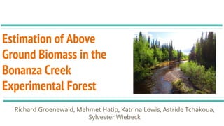
2. Bonanza Creek
Experimental Forest
● Long-Term Ecological
Research (LTER) site within
Tanana Valley Alaska.
● Consists of vegetation and
landforms typical of interior
Alaska.

3. Project Goal
Create a continuous map of predicted
Above Ground Biomass (AGB) with
uncertainty quantification for the
Bonanza Creek Experimental Forest in
interior Alaska.

4. Data
● Forest Inventory Plots data
● G-LiHT LiDAR Plane Data
● LandSat Data

5. Steps Taken
1. Finding and exploring the data
2. Looking for relationships among the variables (AGB, TD and BA) and
covariates (the BGW tasseled cap indices)
3. Coming up with simpler models for a rough estimate, which takes less time.
4. Designing and implementing more complex models
5. Visualizing our model into a continuous map

6. All Relevant Variables
● P10..P100 values
● Tree Density (TD)
● Basal Area (BA)
● Brightness
● Greenness
● Wetness
● Land Cover Type (open water,
deciduous forest, etc.)
● Percent Tree Cover (Hansen)
● Location

7. Predictor Variables of AGB
● TD, BA measured along with AGB, only
on plot land
● Not relevant to measuring AGB on any
point in the map
● P90 and P100 have strong correlation
with AGB, and are measured in a
larger area with the LiDAR sensor
● Likewise, brightness, greenness,
wetness, and percent tree cover
measured everywhere in forest with
satellites

8. Simplified Models
● By basis of comparison, prevents skewed results
● Shows why we need a more complex model
○ They vary in answer because not all the data is considered
○ Instead, approximations are made
The simplest model: Add up the AGB of the 71 plots, multiply that out to
reflect the full forest size.

9. Simplified Model
● Based on simple spatial
model used in Colorado
data tutorial
● Inconsistent, but early
indicator of trends
● Proved necessity for a
more complex model, one
based on multiple
variables

10. Methodology
Let denote AGB and denote a vector of observed
explanatory variables. We model our response as follows:
where and
*Note: assume two error terms are independent.
- Mean function f may be any function of the explanatory variables. Note matrix
of transposed f vectors is our design matrix F
Conditioning as if we know R, we choose a vector c(x) which at unobserved x:

11. Correlation Structure

12. Maximum Likelihood Estimation
Denote
We assume (symmetric) is positive definite and thus invertible
with a Cholesky decomposition (i.e.
for some lower triangular and invertible L)
In this case, the MLE for , assuming R is KNOWN, is:

13. Maximum Likelihood Estimation (Cont.)
We maximize the profile likelihood function:
with respect to the parameters in the covariance matrix [1].

14. Results (Model 1)
Initially fit ordinary least squares stepwise regression to help guess at
covariates to use.
Settled on basic linear combination of P90, brightness, greenness, wetness,
and hansen (% of tree cover)
Imputed 51/284 missing values for P90 using initial spatial regression model.
Used imputations to construct final spatial regression model for AGB.

15. Results (Model 1)
Fitted Model:
Problem:
Note the negative AGB values: this
is an error in the model, possibly
due to imputation issues in P90.

16. Visualization http://rpubs.com/katlewis15/391861

17. Results (Model 2)
Refit without P90 values, this time for entirely
available satellite data:
Fitted model:

18. Model Verification
● We know the exact AGB for the plots, so if our model can predict that
number when we plug in the coordinates, then we are successful
● The satellite covariates give us a low-quality full map, which we can
compare to the map constructed by our model to validate results

19. Challenges faced
● How to account for missing data
● Observed AGB without consideration of tree species, due to limited time
● Large amounts of data caused technological difficulties with laptop
running time

20. Ideas for future work
Cross validation (dividing data into one used to learn or train a model and the
other used to validate the model) to estimate how accurately the predictive model
will perform in practice.
Incorporate uncertainty into the model predictions.

21. Fitting the Puzzle Together
Katrina - Powerpoint design, visualization of data using Leaflet
Richard - Model selection, choosing a covariance structure, obtaining resources
from papers/literature, coding, implementation
Mehmet- Discovering preliminary correlations through R, compiling full data set,
applying R tutorial knowledge in project
Astride - Document the challenges, and ideas for future work on the project.
Implement finishing touches to powerpoint.
Sylvester- Keep team spirits up, simplified models, ideas for future work, and
powerpoint work

22. Special Thanks to
● Statistical and Applied Mathematical Sciences Institute.
● Elvan Ceyhan, Doug Nychka, Chris Jones and Thomas Gehrmann for
organizing and supervising the workshop.
● Andrew Finley for giving us more insight about spatial models as well as
overview of the forest project.
● Huang Huang, our project leader.

23. Citations
1. Sacks, Jerome; Welch, William J.; Mitchell, Toby J.; Wynn, Henry P. Design and Analysis of Computer
Experiments. Statist. Sci. 4 (1989), no. 4, 409--423. doi:10.1214/ss/1177012413.
https://projecteuclid.org/euclid.ss/1177012413
2. Nychka, D., Furrer, R. & Sain, S. 2015. Package “fields.” CRAN.
3. Finley AO, Banerjee S, Carlin BP (2007). “spBayes: An R Package for Univariate and Multivariate Hierarchical
Point-Referenced Spatial Models.” Journal of Statistical Software, 19(4), 1–24. URL
http://www.jstatsoft.org/v19/i04/.
4. Bechtold, W.A. and Patterson, P.L. (2005). The Enhanced Forest Inventory and Analysis Program: National
Sampling Design and Estimation Procedures. US Department of Agriculture Forest Service, Southern Research
Station Asheville, North Carolina.
5. Jakubowski, M.K., Guo, Q., and Kelly, M. (2013). Tradeoffs between lidar pulse density and forest measurement
accuracy. Remote Sensing of Environment, 130, 245-253.
6. White, J.C., Wulder, M.A., Varhola, A., Vastaranta, M., Coops Nicholas, C., Cook, B.D., Pitt, D., and Woods, M.
(2013). A best practices guide for generating forest inventory attributes from airborne laser scanning data
using an area-based approach. The Forestry Chronicle, 89, 722-723.