Electrodynamics

1. From First Principles
PART II – MODERN PHYSICS
May 2017 – R2.1
Maurice R. TREMBLAY
http://atlas.ch
Candidate Higgs
Decay to four
muons recorded by
ATLAS in 2012.
Chapter 1

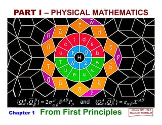
2. 2017
MRT
θθθθo
)(tancos2
),,(
oo
2oo
Lh
L|g|
hLv
−
=
θθ
θ
vo
A project in business and science is a collaborative
enterprise, frequently involving research or design,
that is carefully planned to achieve a ‘particular’ AIM.1
A project is a temporary endeavor to create a ‘unique’
SERVICE.2
1 Oxford English Dictionary
2 PMBOK 4th Edition – Project Management Institute (PMI®)
A
B
αααα
r(t)
dr(t)/dt=v(t)
ZAB
L
h
AB
[ ]
∫≡
B
A
i
ABttZ e)()](),([ vr h
DDDD
ACTION
ACTION
PLAN
MILESTONE
SCOPE
ACTION S
The time t-integral
of the difference
between Kinetic T
(e.g., when a mass
m is in motion) and
Potential V (e.g.,
due to gravity g and
height h) energies:
ACTION
RISK
A Project Manager and a Basketball Shot
DDDDn
EXECUTION2017
PMO
=S ∫
t
o
T−V )( dtt
to
t
g
otan
2
tan θαααα −=
L
h
Basketball
weight: 1.31 lb
diameter: 9.47 in.
Fair=− k v ≅ 0
m
where m is at a
distance L away
and is shot at
an angle θo.
NETWORK
ENGINEERING

3. A Project Manager and Milestones in space-time
MILESTONE #1
MILESTONE #2
MILESTONE S #3 & 4
MILESTONE S #5
DELIVERABLES 3 & 4
DELIVERABLE 2
RISK 2
STAKEHOLDER
SPONSOR
2017
MRT

4. A Field Theorist and a Path Integral in Vn
V2
V5
χχχχ2 >>>>φφφφ2φφφφ †
2
Vi ≡≡≡≡ V0
φφφφ 3,4
V1
Vf <<<< V1
√√√√(½)(V3 ++++V4)
2017
MRT

5. □
Prolog – The Pythagorean† ‘3-4-5’ Theorem
In any ‘right’ triangle*, the area of the square whose side is the hypotenuse c is
equal to the sum of the areas of the squares whose sides are the two legs a and b.
In vector c (or the 4-vector u) notation we write: (direction) _
In scalar c2 ≡ |c|2 (or the invariant ds2 ) notation we write: a2 ⊕ b2 = c2 (magnitude) _
N.B., The Theorem only works in 2-dimensions: a flat table,
a piece of 8.5××××11 paper, &c. In 3 & 4-dimensions, we have
to add depth and interval of light travel…
† Pythagoras, about 572-497 B.C.
*The right angle is indicated by the □. c is the opposite side of the right-angle and a and b are the adjacent sides to this 90° angle
(or π/2 radians). Furthermore, the sum of all the angles (only 3 in a triangle or even 3∠) within the ‘right’ triangle is also equal to 180o.
This slide shows that paying attention to detail in physics is crucial: each letter or symbol
has a meaning – it is a language and it has a meaning which, at times, is far reaching!
≡≡≡≡ ⊕⊕⊕⊕
====
ba
c
cba
rrrrrrrrrrrr
=⊕c
rrrr
2017
MRT
c2
b2a2
O
rrrr
3
45
32
42
52
a
bc

6. cba =+ 22
:Algebra
“The square on the hypotenuse is equal to the sum of the squares on the other
two sides – one adjacent to the right angle and the other opposite.”
With the Pythagorean theorem, x2 +y2 =12 =1×1=1 meter-stick long (a metric reference
frame), we have cos2θ +sin2θ =1 or with exp(Im(t))=eiθ =cosθ +isinθ we get eiπ +1=0
when θ =π≡PI() ≅ 3.141592…………=180° and i=√(−1) is the complex number and i=eiπ/2.
222
cba =+:Algebra
a
bc
ADJACENT
OPPOSITE
2017
MRT
If we let cbe the length of the hypotenuse
and a and b be the lengths of the other
two sides, the theorem can be expressed
as the algebraic (latin: algebra) equation:
or, solved for c (i.e., using the square-root
symbol – i.e., “√ ” which is the inverse “…2”
function of squaring things – i.e., Einstein’s
Mass-Energy formula: E = m‘c2’):
or, using a=3 and b=4, we get:
32+42=(3×3)+(4×4)=9+16=25
32+42=52⇒√(9+16)=√(25)=5

7. θθ coscos ⋅=⇒=== ca
c
a
eHypothenus
sideAdjacent
Cosine
θθ sinsin ⋅=⇒=== cb
c
b
eHypothenus
sideOpposite
Sine
a
b
a
b
c
a
c
b
=⋅=====
c
cθ
θ
θ
cos
sin
tan
sideAdjacent
sideOpposite
Tangent
1sincos 22
=+ θθ
Now, the equation:
a2 +b2 =c2
will give with the above:
Here’s a rough proof:
Dividing each term by c gives us cos2θ +sin2θ =1.
√[(c⋅cosθ )2 +(c⋅sinθ )2]=√[(c)2⋅(cosθ )2 +(c)2⋅(sinθ )2]=√[c2⋅(cos2θ +sin2θ )]=√[c2⋅(1)]
=√(c2)=
=c With emphasis to show that “ √ ” is the inverse function of “ …2 ” because in they end, they nullify each other.
Definitions: Sym. Name Ratio of… (i.e., side a divided by side c)
2
c
2017
MRT
a
bc
OPPOSITE
ADJACENT
θ
c⋅sinθ
c⋅cosθ
Hence:
If:
and

8. The diagram can serve as a useful mnemonic for remembering the above relations
involving relativistic energy E, rest mass mo, and relativistic momentum p [N.B., the nota-
tion used in this diagram is: the invariant rest mass is subscripted with a naught ‘o’, mo
(whereas the relativistic mass is m), T is the energy due to motion – the kinetic energy.]
Most of the
particle’s
energy is
contained in its
rest mass, mo
22
)(
2
o
2
42
o
22
mcEcm
c
p
cmcpE
m
=⇔








+





=+=⇒
massicrelativist
)18090( oo
=++φθ
c
p
om
m
22
o
22
)()( cmpcE ⊕≡
22
o mccmTE =⊕≡
1) E is the sum of the kinetic T and rest-mass moc2 energies, 2) the square of the
relativistic energy E (i.e., E2 in the Figure), is also equal to the sum of the square of
the relativistic momentum energy pc and the square of the rest-mass energy moc2.
2
o )( cmmT −=where
Energy required (in the
form of motion) to bring
the mass mo from rest
to a given momentum p.
2017
MRT (moc)c =moc2
pc

9. D
V
This is a galaxy located 1.5
Mpc away receding from
our galaxy with a velocity of
110 km/s giving Ho = V /D =
73 km/s/Mpc.
1442443144244314424431442443












Ho = 73 km/s/Mpc
Hubble’s Law: Velocity = [Slope] ×××× Distance
Again, in the language of math
(i.e., in an algebraic equation):
y ==== m × x + 0000
where y is the observed velocity
of the galaxy away from us,
usually in km/s. m, the slope, is a
“Constant” – the slope of the
graph – here in km/s/Mpc. x is the
distance to the galaxy in Mpc.
Finally, given any m, with x = 0 we
have y = 0, then b = 0 (see Graph).
Ho = 50 km/s/Mpc
Velocity(km/s)
Distance (Mpc / 1××××106 parsec)
=
D
V
Ho
2017
MRT

10. The dominant motion in the universe is the smooth expansion known as Hubble’s Law.
Recessional Velocity of a Galaxy = Hubble’s Constant × Distance
In 1929, Hubble estimated the
value of the expansion factor, now
called the Hubble constant, to be
about Ho ∼50 km/s/Mpc. Today the
value is still rather uncertain, but is
generally believed to be in the
range of Ho ∼45-90 km/s/Mpc.
In the language of Physics (i.e., a
mathematical law representing a
true observable phenomenon):
V====Ho×D
V is the observed velocity of the
galaxy away from us, usually in
km/s. Ho is Hubble’s “Constant”, in
km/s/Mpc. D is the distance to the
galaxy in Mpc (1 Mpc∼3×1022 m)
Velocity(km/s)
Distance (Mpc / 1××××106 parsec)
2017
MRT

11. 2017
MRT
Forward
This is a slideshow on the fundamental theoretical ideas and techniques of Modern Physics– those embo-
died in special relativity and the quantum hypothesis as formulated using matter waves. The emphasis is
on the mathematical formulation of fundamentalideas,together with the illustrative calculations to show how
the theory is used in obtaining quantities that can be checked against experiment (c.f., References), there-
by demonstrating that the theory is believable.Most of the theory is developed in several dimensions (e.g.,
at position r =xi) because the common person lives in three space dimensions; it is intended that he or she
should see immediately how the theory is applicable in three- (and four-) dimensional problems (e.g., xµ).
With the above in mind, the first five chapters of this work have managed to compile a modern, while
very brief, Review of Electromagnetism beginning from the experimental laws of Coulomb and Biot-
Savart, later introducing Faraday’s law of electromagnetic induction, and culminating in Maxwell’s equa-
tions and the wave equations for electromagnetic field quantities. This sets the stage for the failure of
Galilean invariance in electromagnetic theory and the consequent fundamental disagreement between
classical mechanics and electromagnetic theory. This review necessarily is brief and is not appropriate as
an introduction to electromagnetic theory. Rather it is intended to set the stage for the work and fun that is
to come, and to orient the reader to a point of view that the author believes to be particularly useful.
11
In succeeding chapters, special relativity and its tensor formulation is built-up from scratch. Then, the
tensor formulation of electromagnetism is developed as an application of the generally-covariant view of
things, as are techniques for handling the kinetics of collision problems. In particular, the energy E and
momentum P (densities) of the electromagnetic field are obtained from the four-dimensional formulation.
Knowing the energy and momentum densities of the electromagnetic field, one can proceed naturally to
the investigation of the spectral distribution I(k) of blackbody radiation. Planck’s law is found in a rather
conventional manner and then we consider briefly such topics as the photoelectric effect, Compton col-
lisions, Rutherford scattering and the Bohr atom. The purpose of this slideshow is primarily for the benefit
of undergraduates and some know-it-alls who have had only a college-level introduction to modern physics.
Lastly, we discuss the behavior of waves in general such as to provide the basis for the introduction
to matter waves and we stop before Born and Heisenberg publish their version of quantum mechanics.

12. Contents of 3-Chapter PART II
PART II – MODERN PHYSICS
Charge and Current Densities
Electromagnetic Induction
Electromagnetic Potentials
Gauge Invariance
Maxwell’s Equations
Foundations of Special Relativity
Tensors of Rank One
4D Formulation of Electromagnetism
Plane Wave Solutions of the Wave
Equation
Special Relativity and
Electromagnetism
The Special Lorentz Transformations
Relativistic Kinematics
Tensors in General
The Metric Tensor
The Problem of Radiation in
Enclosures
Thermodynamic Considerations
2017
MRT
The Wien Displacement Law
The Rayleigh-Jeans Law
Planck’s Resolution of the Problem
Photons and Electrons
Scattering Problems
The Rutherford Cross-Section
Bohr’s Model
Fundamental Properties of Waves
The Hypothesis of de Broglie and Einstein
Appendix: The General Theory of
Relativity
References
“I think that modern physics has definitely decided in favor of Plato. In fact the smallest units of matter
are not physical objects in the ordinary sense; they are forms, ideas which can be expressed
unambiguously only in mathematical language.” Werner Heisenberg
12

13. Contents
PART II – MODERN PHYSICS
Charge and Current Densities
Electromagnetic Induction
Electromagnetic Potentials
Gauge Invariance
Maxwell’s Equations
Foundations of Special Relativity
Tensors of Rank One
4D Formulation of Electromagnetism
Plane Wave Solutions of the Wave
Equation
Special Relativity and
Electromagnetism
The Special Lorentz Transformations
Relativistic Kinematics
Tensors in General
The Metric Tensor
The Problem of Radiation in
Enclosures
Thermodynamic Considerations
2017
MRT
The Wien Displacement Law
The Rayleigh-Jeans Law
Planck’s Resolution of the Problem
Photons and Electrons
Scattering Problems
The Rutherford Cross-Section
Bohr’s Model
Fundamental Properties of Waves
The Hypothesis of de Broglie and Einstein
Appendix: The General Theory of
Relativity
References
13

14. We find, experimentally, that the ‘force’ that acts on an arbitrary ‘charge’ – however
many there are or how many that are moving – depends only on the position of this
charge, its velocity and the quantity of charge. We can write the (resultant) force F
on this charge q moving with velocity v by the Lorentz force law:
F=q(E+v××××B)=qE⊕qv××××B (Electric force ⊕ Magnetic force)
Within electromagnetism, a ‘field’ is a physical quantity that takes different values at
different points of space. We consider a static (dynamic) field then as a mathematical
function of space (space and time) and to visualize this field we draw many points in a
3D space and at each should be given the intensity and direction of the vector field at that
location. As we step back and look over the space, the field is then defined and mapped
physically – it has become a manifold – and it will help provide a representation that
will be done using some advanced mathematical concepts which we will turn to next.
where we call E the electric field and B the magnetic field at the position (e.g., in simple
Cartesian coordinatesx, y & z) of the charge q(x,y,z). We can think of E(x,y,z) and B(x,y,z)
as producing the forces that can be seen at a time t by charge q situated at [x,y,z] with
the condition that: having placed the charge in its place it is not perturbed any further!!!
We also associate with any coordinate [x,y,z] of space two physical orientated quan-
tities (i.e., vectors), E and B, that can vary with time t. The electric and magnetic fields
are then visualized as vector functions of x, y, z and t. Since a vector is specified by its
components, each of the fields E(x,y,z,t) and B(x,y,z,t) represents three mathematical
functions of x, y, z and t. We will now generally refer to the position vector r (e.g.,[x,y,z]).
2017
MRT
14
Charge and Current Densities

15. •
y
x
z
E
Electric Vector
Field Lines (i.e.,
force field per
unit charge)
Manifold
of coupling
kE
R
r
r
r rR= rrR=⇒
R= R Rˆ=R Rˆ
R
rr −−−−
=Rˆ
( )





 −+−+−==∝=
==∝
+−+−+−
222
22
32
)()()()(
)()(
zzyyxx
R
Q
k
Q
F
Q
k
Q
R
R
rF
RRrr
rrR
rF
E
E −−−−
−−−−
Three-dimensional space representation of the
interaction of two point charges Q=+q and q =−q,
the distance R=|R| & kE is Coulomb’s constant.
2017
MRT
Also, R = r−−−−r is the separation distance and kE is a
proportionality constant – a positive force implies it is
repulsive, while a negative force implies it is attractive. The
proportionality constant (i.e., the coupling intensity between
charges) kE, called the Coulomb constant, is related to
defined properties of space and can be calculated based on
knowledge of empirical measurements of the speed of light:
22
/CoulombmeterNewton
rHenry/mete
⋅×=
×=== −
9
72
2
o
o
10987.8
10
π4
µ
επ4
1
c
c
kE
Direction:
Magnitude:
So, by experience, we know that a force that either attracts or repels will be exerted on a
test charge q when it is placed in the vicinity of another point charge Q. Mathematically:
This force acts at a distance R=|R| away (in the direction of a unit vector parallel to R).Rˆ
To aid in visualizing the E field, we introduce the ‘concept’
of field lines (see Figure) which gives the direction of the
electrical force generated by a positive test charge (e.g., Q =
+q in Figure). If another test charge was released (e.g., q=−q
in Figure), it would move in the direction of the field lines.
15
q q
qq
Rˆ Rˆ
−−−−
++++
Q
r
r
Rˆ
O
q
rrR=
Source
Sink
2 point charges
withnodimensions

16. Now, let us demonstrate a specific mathematical representation of the three-dimen-
sional δ -function, δ 3(r). By direct differentiation, one obtains, for a radius vector r ≠r:
2017
MRT
0
)(
3
1
3
1
)()(
1
)()(
1
5
2
333
3
212
=








−−=








•+•−=
•−=−•=•≡∇
−−
rr
rr
rrrr
rrrr
rr
rr
rr
rrrr
rr
−−−−
−−−−
−−−−−−−−
∇∇∇∇−−−−−−−−∇∇∇∇
−−−−
−−−−
−−−−
∇∇∇∇−−−−∇∇∇∇−−−−∇∇∇∇∇∇∇∇
−−−−
hence ∇2(1/|r−−−−r|) satisfies δ 3(r)=0 (if r≠0), which is the first property of a δ -function!
Also, if r lies outside a region having volume V and enclosed by a surface S, then:
16
0
1 32
=∇∫∫∫V
d r
rr −−−−
because r≠r for every vector r contained in V, and hence ∇2(1/|r−−−−r|) vanishes
everywhere in V. On the other hand, if V is chosen so that it contains r, we have:
∫∫∫∫∫∫∫∫∫∫ •−=•=•=∇
SSVV
dddd S
rr
rr
Srr
rr 3
332 1
−−−−
−−−−
∇∇∇∇
−−−−
Gauss
according to Gauss’s theorem (i.e., for a vector F=∇∇∇∇(1/|r−r|)) for the gradient of |r−−−−r|−1:
∫∫∫∫∫ •=•
VS
dd rFSF 3
∇∇∇∇
1
| r −−−− r |
_∇∇∇∇
1
| r −−−− r |
_∇∇∇∇

17. Now, let us choose a small sphere centered at r, having volume V and surface S, and
contained entirely within V. Since ∇2(1/|r−r|)=0 everywhere within the volume V−V (i.e.,
everywhere within V but outside of V ), we have:
17
2017
MRT
0
11 3232
=∇−∇ ∫∫∫∫∫∫ VV
dd r
rr
r
rr −−−−−−−−
but:
π4
sin)(
1 π2
0
π
033
32
−=
−=Ω−=Ω•−=•−=∇ ∫ ∫∫∫∫∫∫∫∫∫∫ θθϕ dddddd
SS
d
SV 44 344 21
S
rrrr
rr
rr
S
rr
rr
r
rr
−−−−−−−−
−−−−
−−−−
−−−−
−−−−
−−−−
where dΩ=sinθ dθ dϕ is an element of solid angle about the point r. This result,
combined with ∫∫∫V∇2(1/|r−r|)d3r−−−− ∫∫∫V∇2(1/|r−r|)d3r=0 above leads to:
π4
1 32
−=∇∫∫∫V
d r
rr −−−−
if r is within V. Therefore, −(1/4π)∇2(1/|r−r|) possesses properties δ 3(r)=0 (if r≠0) and
∫∫∫V-δ 3(r)d3r=1 (if r=0 is in volume V ) and =0 (if r=0 is not in volume V ), we obtain:
)(
1
π4
1 32
rr
rr
−−−−
−−−−
δ≡∇−
This representation of the three-dimensional δ -function is particularly useful in
the investigation of electromagnetic fields. One last property of the δ -function is
∫∫∫V-δ 3(r) f (r)d3r= f (0) (if r=0 is in volume V ).

18. Q q
E
FC
++++q1 −−−−q2
v(r) = 0
Gaussian
Surface
Point charge Q = +q1 attracts q = −q2.
)(3
1
2
C
rr
rr
F
E E −−−−
−−−−
q
k
q
=−=
Coulomb’s Law (Charles Coulomb – 1783): The magnitude
of the ‘electrostatic’ force of interaction between two point
charges is directly proportional to the scalar multiplication
of the magnitudes of charges and inversely proportional to
the square of the distances between them. (wikipedia.org)
The scalar form of Coulomb’s law is an expression for the magnitude and sign of the electrostatic force between
two idealized point charges, small in size compared to their separation. This force (FC) acting simultaneously on
point charges (Q=+q1) and (q=−q2), is given by:
2
21
2
12
CC
3C
)(
)()(
rrrr
rF
rr
rr
rF
EE
E
−−−−−−−−
−−−−
−−−−
qq
k
qq
kF
Qq
k
−=
+−
==
=
•
Illustration of the electric field surrounding a
positive (red) and a negative (blue) charge.
Direction:
Magnitude:
2017
MRT
r −−−− r
++++q1 ++++q2
++++q1 −−−−q2
Q = +q1
attracts
q = −q2
Q = +q1
repels
q = +q2
2
2
2
2
1
C
1
C
3
C
)(
)(
)(
)(
)(
rrrr
rF
rE
rr
rr
rF
rE
EE
E
−−−−−−−−
−−−−
−−−−
q
k
q
k
q
F
q
E
Q
k
q
−=
−
==
+
==
==
The direction of the electric field vector E is (always) from
the positive to the negative charge whereas the magnitude
of the electric field E=|E| at a point is the force per unit
charge on a positive test charge at the point:
kE(εo)
Field
18

19. Flux ΦE through a spherical (Gaussian) surface
of radius r (ASphere = 4πr2) from an electric field
with at it center a point positive charge Q.
Gauss’s law also has a differential form:
∫∫∫=
V
dddrrQ ϕθθρ sin)( 2
r
Gauss’s Law (Carl Gauss – 1834): The electric flux
through any closed surface is proportional to (i.e.,
‘∝∝∝∝’) the enclosed electric charge. (wikipedia.org)
ϕθθ
θ
θ
ρ ϕθ
∂
∂
+
∂
∂
+
∂
∂
=•=
E
r
E
rr
Er
r
r
sin
1)sin(
sin
1)(1
ε
2
2
o
E∇∇∇∇
where ∇∇∇∇•E is the divergence of the electric field, and ρ is
the charge density. The electric flux ΦE through any closed
(e.g., an arbitrary spherical) surface due to a point charge Q
can be written as:
oε
Q
d
S
=•=Φ ∫∫ SEE
Gauss’s Law states that the (net) electric flux through any closed surface is equal to the charge inside
that surface divided by the dielectric constant εo. Gauss’s Law may be expressed in its integral form:
Qd
S
∝•∫∫ SE
Here ΦE =∫∫S E•dS is a surface integral denoting the
electric flux through a closed surface S and Q denotes the
total charge enclosed by volume V :
(Spherical Coordinates)
2017
MRT
rE ˆ
επ4
1
2
o r
Q
=
Gaussian
Surface
dS
dΦEQ
r
Constant electrical
field lines
r
r
r=ˆ
rS ˆπ4 2
rd =
Er
r
EdrrErdrErdEdQ
r
rr
S
2
o
0
2
o
0
o
0
o
2
oo επ4
2
επ8επ8)π8()ˆˆ(ε)ˆπ4()ˆ(εε =⋅=⋅=•=•=•= ∫∫∫∫∫ rrrrSE
19

20. This Figure shows the velocity (dv) induced at
a point P by an element of vortex filament (dllll)
of strength Γ.
Biot–Savart’s Law (J.-B. Biot & F. Savart – 1820): The magnetic vector field B de-
pends on the magnitude, direction, length, and ‘proximity’ of the electric current I,
and also on a fundamental constant called the magnetic constant µo. (wikipedia.org)
With the definition of the current, I=J • S, the law is:
where the integral sums over the wire length where vector
dllll is the direction of the current, µo is the magnetic
constant, r−−−−r is the distance between the location of the
infinitesimal length dllll and the location at which the
magnetic field is being calculated.
∫=
rr
rr
B
−−−−
−−−−×××× )(
π4
µo l
r
dI
The Biot-Savart Law is used to compute the magnetic field generated by a steady
current (i.e., a continual flow of charge – e.g., through 1m long 18-gauge copper
speaker wire − which is constant in time and in which charge is neither building up nor
depleting at any point).
Enclosedoµ Id
C
=•∫ l
r
B
where the line integral is over any arbitrary loop and IEnclosed
is the current enclosed by that loop.
dllll
P
dv
r − r
dfBS
2017
MRT
Vortex filament of strength Γ
A slightly more general way of relating the current I to the
magnetic field B is through Ampère's Law:








= 3
o
BS
)(
)(
π4
)(µ
)(
rr
rr
rv
r
rf
−−−−
−−−−××××
××××
l
r
dI
d
ρ
20

21. The relation between the current density J
(current per unit area) and the current I in a
cylindrical conductor (with conductivity σ ).
A familiar example of a current density is that in a
cylindrical conductor (say a wire of conductivity σ ) having
radius r and carrying a constant current I, i.e., is the amount
of charge transferred across the conductor's cross sectional
surfaces per unit time:
One could express the density current J(r) and a velocity distribution v(r) if the
velocity of each element of charge at each point in space (not time as in space-time
which would greatly complicate things!) were known; thus one would have:
vS
I
vSt
Q
tSvtvSVQ
vv
vJ
∆
=
∆






∆
∆
==∴
∆∆=∆∆=∆=∆
1
][
ρ
ρρρ
)(ˆlim)()()(
0
0
rJrvrrJ
tS
Q
t
S ∆∆
∆
==
→∆
→∆
ρ
)()()( rvrrJ ρ=
Knowing J(r) is equivalent to knowing v(r) if ρ (r) is given and it is more convenient to
work with the current density than with the velocity distribution. J=ρ v gives us a notion
of the meaning of J(r): it is the amount of charge ∆Q passing across a surface ∆S
perpendicular to J (and therefore also to v) at the position r during time interval ∆t – as
∆S and ∆Q tend to vanish (that ‘ → 0’ symbol):
2
2
π
π)(
r
I
J
rJd
td
dQ
I
S
=
=•== ∫ SrJ
2017
MRT
J
Sr
σσσσ
y
x
z v
∆∆∆∆S
O
Wire
v∆∆∆∆t
r
tQ
rJSJI
rS
∆∆=
==
=
2
2
π
π
In a nutshell, the ‘electric’ current is the rate of flow of
electric charge.
21

22. Now, we shall consider two of the fundamental laws of electromagnetism,Coulomb’s
law and the law of Biot and Savart. A mathematical generalization of the experimental
facts is given in the following two expressions for the force per unit volume experienced
by an electric charge density ρ(r), and an electric current density J(r), respectively:
22
2017
MRT
∫∫∫=
V
d r
rr
rr
rrf 3
3
o
C )()(
επ4
1
−−−−
−−−−
ρρ
where fC (r) is the force density arising from the ‘static’ distribution of charges (i.e., qE),
fBS (r) is the force density attributable to ‘moving’ charges or currents (i.e., qv××××B), and εo
and µo represent experimental constants characterizing the permittivity and permeability
of the free space (i.e., in a total vacuum which is space void of matter). Thus, the total
electromagnetic force arising from a static system of charges or from currents is then:
∫∫∫=
V
d rrfrF 3
BSC,BSC, )()(
where the integration is carried out over the volume V containing the system of electric
charges. Since ρ(r) is the charge per unit volume, the total charge in volume V is:
∫∫∫=
V
dQ rr 3
)(ρ
∫∫∫=
V
d r
rr
rr
rJrJf 3
3
o
BS )(ˆ)(
π4
µ
−−−−
−−−−
××××××××
and

23. Force due to charge in motion (v ≠ 0):
Force due to charge at rest (static):
Consider an application where we are situated at an origin O of a reference frame S
(i.e., aCartesianCoordinateReferenceFrame) that has volume V. Consider also an other
reference frame S (i.e., a spherically symmetric Gaussian Surface or even equipotential
flow or vortex lines) also with it’s own origin O which can be quite a distance r away from O.
Coordinate system used to describe the density
of force at point P. Both the densities of charge
ρ(r) and current J(r) generate from O the E(r)
and B(r) fields at point P from a distance r − r
away – and measured a distance r from O.
(Biot-Savart’s Law)








−
−
= ∫∫∫V
d r
rr
rrrJ
rJrf 3
3
o
BS
)()(ˆ
)(
π4
µ
)(
××××
××××
(Coulomb’s Law)
∫∫∫ −
−
=
V
d r
rr
rrr
rrf 3
3
o
C
))((
)(
επ4
1
)(
ρ
ρ
fC is thus the force density arising from a ‘static’ distribution
of charges whereas fBS is the force density attributable to
‘moving’ charges or currents and the permittivity of free space
(the dielectric constant) εo and permeability of free space (or
magnetic constant) µo are respectively given by:
εo = 8.854×10−12 Faraday/meter
µo = 4π ×10−7 Newton/Ampere2
2017
MRT
ˆ
As a reference, the current I at P′ is given by:
I = J • S
We then do – from O – an observation of the force densities a distance r away at point P (e.g., produced within
O by a density of charge ρ and current J ) situated at a distance r −−−− r away from O. A mathematical generalization
of the experimental facts is given by the two following expressions for the force per unit volume V felt by an
electrical charge density ρ(r) and an electrical current density J(r) (in the direction of the unit vector J /|J|):
•
y
x
z
)(rJ
)(rJ)(rρ
O
P′
)(rv
O
r –
r
)(rρ
r
rr++++
−
Gaussian
Surface
Flow
Line
P
ˆ
23

24. )()()()()()( BSC rBrJrfrErrf ××××== andρ
or, evidently, after wrapping everything with an integral over the whole volume V in S :
∫∫∫∫∫∫ −
−
=
−
−
=
VV
dd r
rr
rr
rJrBr
rr
rr
rrE 3
3
o3
3
o
)(ˆ
π4
µ
)()(
επ4
1
)( ××××andρ
It is convenient to express the force densities as functions of the two vector fields: the
electrical field E(r) and the magnetic field B(r). The relation between the densities of
force and the vector fields is given by (notice how the density – i.e., the amount per unit
volume – of charge ρ and of current J factor into the definition of fC(r) and fBS(r)):
rrrr
rr
−
−=
−
− 1
3
∇∇∇∇
2017
MRT
53
3
1
rr
rr
rr −
−
−=
−
∇∇∇∇&
With the unit vector = J/|J| parallel and normal to a unit
element of the surface (e.g., a sphere) through which the
vector representing the current density would pass and these
relations will provide benefit as variation representations:
The undisturbed charge q will be subject to E(r)
and B(r) in proportion to both the densities of
charge ρ(r) and current J(r) at point P, r away
from O and r −−−− r away from O. The velocity v(r)
factors in for F(v)= qE⊕qv××××B and J(v) = ρv.
Since ρ (r) is the charge per unit volume, the total charge in
volume V (e.g., in spherical coordinates):
where the (e.g., spherical again) gradient ∇∇∇∇ is given by:
∫∫∫=
V
drddrrq
Spherical
2
sin),,( ϕθθϕθρ
ϕϕϕϕ∇∇∇∇ ˆ
sin
1ˆ1
ˆ
ϕθθ ∂
∂
+
∂
∂
+
∂
∂
=
rrr
θry
z
)(rJ)rρ
)(rv
q
q
Charge
(
−
)(rJ
)(rρ
)(ˆ rrJ −´
q
)(rJ
)(rρ
ˆ
•
x
)(rJ
)(rρ
r Q
Jˆ
J )
)
J
++++ rr
ˆ
r
P′
)(rρ
)(rBˆ(r ××××
(E r
)(rfC )(rfBS
P
24

25. Now, by using the vector identity ∇∇∇∇•(U××××V)=V•(∇∇∇∇××××U)−U•(∇∇∇∇××××V), we can at first find
the divergences of E(r)=(1/4πεo)∫∫∫V ρ(r)[(r−−−−r)/|r−−−−r|3]d3r:
25
2017
MRT
)(
ε
1
)()(
ε
11
π4
1
)(
ε
1
1
)(
επ4
11
)(
επ4
1
o
33
o
32
o
32
o
3
o
rrrrrr
rr
r
r
rr
rr
rr
rE
ρδρρ
ρρ
=−=∇−=
∇−=•−=•
∫∫∫∫∫∫
∫∫∫∫∫∫
VV
VV
dd
dd
−−−−
−−−−
−−−−−−−−
∇∇∇∇∇∇∇∇∇∇∇∇
where we have used the fact that ∇∇∇∇g(x−−−−x)=−∇∇∇∇ g(x−−−−x) when ∇∇∇∇ means differentiation with
respect to three-dimensional Cartesian coordinates x (or r if three-dimensional Spherical
coordinates are used), such that ∇∇∇∇=−Σj xj∂/∂xj and ∇∇∇∇=−Σj xj∂/∂xj where j =1,2,3 and ∇∇∇∇
means differentiation with respect to x). Second, for B(r)=(µo/4π)∫∫∫V J(r)××××[(r−−−−r)/|r −−−−r|3]d3r:
0
1
)(
π4
µ
1
)(
π4
µ1
)(
π4
µ
3o
3o3o
=








•−=








•−=•−=•
∫∫∫
∫∫∫∫∫∫
V
VV
d
dd
r
rr
rJ
r
rr
rJr
rr
rJB
−−−−
∇∇∇∇××××∇∇∇∇
−−−−
∇∇∇∇××××∇∇∇∇
−−−−
∇∇∇∇××××∇∇∇∇∇∇∇∇
ˆ ˆ
These last divergences are two of Maxwell’s differential equations for the
electromagnetic fields in vacua:
0)(
ε
1
o
=•=• BrE ∇∇∇∇∇∇∇∇ andρ
ˆ

26. Compasses reveal the direction of the local
magnetic field. As seen here, the magnetic
field points towards a magnet’s S (south) pole
and away from its N (north) pole.
B B
B field lines never end! Magnetic field lines exit a magnet near its north pole and
enter near its south pole, but inside the magnet B field lines continue through the mag-
net from the south pole back to the north. If a B field line enters a magnet somewhere it
has to leave somewhere else; it is not allowed to have an end point. Magnetic poles,
therefore, always come in N (North) and S (South) pairs. Cutting a magnet in half results
in two separate magnets each with both a north and a south pole. (wikipedia.org)
Since all the magnetic field lines that enter any given
region must also leave that region, subtracting the ‘number’
of field lines that enter the region from the number that exit
gives identically zero.
Conceptually thinking, this is equivalent to saying that the
magnetic flux ΦB through any closed surface S is identically
zero, and mathematically it is equivalent to the integral
form:
where the integral is a surface integral over the closed
surface S (a closed surface is one that completely surrounds
a region with no holes to let any field lines escape). Since dS
points outward, the dot product in the integral is positive for
B field pointing out and negative for B field pointing in. It
also has a differential form:
2017
MRT 0
sin
1)sin(
sin
1)(1 2
2
=
∂
∂
+
∂
∂
+
∂
∂
=•
ϕθθ
θ
θ
ϕθ
B
r
B
rr
Br
r
r
B∇∇∇∇
0=•=Φ ∫∫S
dSBB
26

27. We can obtain another pair of differential equations for E(r) and B(r) by calculating
their curls. Taking the curl of E(r)=(1/4πεo)∫∫∫V ρ(r)[(r−−−−r)/|r−−−−r|3]d3r yields:
27
2017
MRT
0r
rr
rE =−= ∫∫∫V
d3
o
1
)(
επ4
1
−−−−
∇∇∇∇××××∇∇∇∇××××∇∇∇∇ ρ
This is interesting! The curl of an electrostatic field is zero, ∇∇∇∇××××E=0!








•+=








•−−=








•+•








•+∇−=








−=
∫∫∫
∫∫∫
∫∫∫
∫∫∫
V
V
V
V
d
d
d
d
r
rr
rJ
rJ
r
rr
rJrJrr
r
rr
rJrJrJ
rrrr
r
rr
rJB
3o
o
33o
32o
3o
)(
π4
µ
)(µ
1
)()()(π4
π4
µ
1
])()([)(
11
π4
µ
1
)(
π4
µ
−−−−
∇∇∇∇∇∇∇∇
−−−−
∇∇∇∇∇∇∇∇−−−−−−−−
−−−−
∇∇∇∇∇∇∇∇∇∇∇∇−−−−∇∇∇∇
−−−−
∇∇∇∇
−−−−
−−−−
∇∇∇∇××××××××∇∇∇∇××××∇∇∇∇
δ
In calculating the curl of B(r)=(µo/4π) ∫∫∫V J(r)××××[(r−−−−r)/|r−−−−r|3]d3r, we must make use of
the vector identity ∇∇∇∇××××(U××××V)=U(∇∇∇∇•V)−V(∇∇∇∇•U)++++(V•∇∇∇∇)U−(U•∇∇∇∇)V, together with the fact
that U•∇∇∇∇J(r)=0 and ∇∇∇∇•J(r)=0 since J(r) does not depend on the variable r. Thus:
ˆ

28. Now, the divergence appearing in the last term (i.e., ∫∫∫V ∇∇∇∇•[J(r)/|r−−−−r|]d3r) can be
rewritten in such a way that we can make use of Gauss’s theorem:
28
2017
MRT
where S is the surface enclosing volume V. If we are realistic in our assumptions about
J(r) for an arbitrary physical problem, we shall require the volume of integration V to be
so large that it encompasses the entire region over which the current density is non-
vanishing, and the J(r) will vanish everywhere on S such that − ∫∫S [J (r)/|r −−−− r|] • dS = 0.
Then we are left with:
∫∫∫∫∫
∫∫∫
∫∫∫∫∫∫∫∫∫
•
•−=








•








•−=
•−=•=•
VS
V
VVV
dd
d
ddd
r
rr
rJ
S
rr
rJ
rrJ
rrrr
rJ
r
rr
rJr
rr
rJr
rr
rJ
3
3
333
)()(
)(
1)(
1
)(
1
)(
)(
−−−−
∇∇∇∇
++++
−−−−
∇∇∇∇
−−−−
−−−−
−−−−
∇∇∇∇
−−−−
∇∇∇∇
−−−−
∇∇∇∇
−−−−
∇∇∇∇
∫∫∫∫∫ •=•
SV
dd SFrF 3
∇∇∇∇
as follows:
0








= ∫∫∫V
d r
rr
rJB 3o
o
π4
µ
)(µ
−−−−
∇∇∇∇++++××××∇∇∇∇
∇∇∇∇ •J(r)
____
−−−−

29. This result can be cast into an even more useful form if we take into account another
very important piece of experimental information, namely the law of conservation of
electric charge. A vast amount of accumulated experimental data supports the
hypothesis that electric charge cannot be created or destroyed spontaneously within a
closed physical system; this circumstance can be expressed mathematically by the
continuity equation:
29
2017
MRT
tt ∂
∂
−=•∇=
∂
∂
+•∇
)(
)(0
)(
)(
r
rJ
r
rJ
ρρ
or
which means that the current density emerging from a point in space (i.e., ∇∇∇∇•J(r)) is
equal to the rate of decrease of the charge density at this point (i.e., −∂ρ(r)/∂t).
However, if J(r) is independent of time, ρ(r), according to the continuity equation above,
will be a linear function of time. This additional experimental information allows us to
replace ∇∇∇∇•J(r) in the above expressions for ∇∇∇∇××××B(r) with −∂ρ(r)/∂t; thus:








∂
∂
=








∂
∂
= ∫∫∫∫∫∫ VV
d
t
d
t
r
rr
rrJr
rr
r
rJB 3o
o
3o
o
1
)(
π4
µ
)(µ
)(
π4
µ
)(µ
−−−−
∇∇∇∇−−−−
−−−−
∇∇∇∇−−−−××××∇∇∇∇ ρ
ρ
of, if we make use of the definition of E(r)=(1/4πεo)∫∫∫V ρ(r)[(r−−−−r)/|r −−−−r|3]d3r:
)(µo rJB =××××∇∇∇∇
The second term (i.e., −µoεo∂E/∂t) represents the so-called displacement current
discovered by Maxwell.
− µo εo
∂ E
∂t

30. dV
V
S
Sdd nS ˆ=
J(r)
y
x
z
r
O
Gauss’ Divergence Theorem: The closed
manifold dV is the boundary of V oriented by
outward-pointing normals, and n is the outward
pointing unit normal field of the boundary dV.
Another important piece of experimental information in which a vast amount of
accumulated experimental data supports the hypothesis that electrical charges cannot
be created or destroyed spontaneously within a closed physical system – this embodies
the Law of conservation of electrical charge and can be expressed mathematically by
the continuity equation:
(The Continuity Equation)
The outward flux of a vector field through a closed surface is
equal to the volume integral of the divergence of the region
inside the surface. Intuitively, it states that the sum of all
sources minus the sum of all sinks gives the net flow out of a
region.
Law of conservation of electrical charge (Benjamin Franklin – 1747): Change in the
amount of electric charge in any volume of space is exactly equal to the amount
of charge flowing into the volume minus the amount of charge flowing out of the
volume. (wikipedia.org)
J•−=
∂
∂
∇∇∇∇
t
ρ
The continuity equation means that the current density
emerging from a point in space (∇∇∇∇•J) is equal to the rate of
decrease of the charge density at that point (−∂ρ/∂t).
Continuity equations offer more examples of laws with both
differential and integral forms, related to each other by the
divergence theorem:
∫∫∫∫∫∫∫ •≡•=•
VSS
dVdSd JnJSJ ∇∇∇∇ˆ
2017
MRT
nˆ
t∂
∂
−=•
)(
)(
r
rJ
ρ
∇∇∇∇
30

31. The set of differential equations we have obtained so far (i.e., ∇∇∇∇•E(r) =(1/εo)ρ(r), ∇∇∇∇•B(r)
=0, ∇∇∇∇××××E(r)=0 – the electric field associated with a set of stationary charges has a curl of
zero there is no magnetic field so ∂B(r)/∂t=0 – and ∇∇∇∇××××B(r) =µoJ(r)++++ µoεo∂E(r)/∂t) still
does not contain all the experimental information about electro-magnetic fields that is
available to us; we have said nothing about Faraday’s law of electromagnetic
induction. The ∇∇∇∇××××E(r)=0 equation above is, in fact, in disagreement with experiment,
as Michael Faraday found during the mid-nineteenth century. He noted first that a closed
loop of conducting material placed in static external electric and magnetic fields did not
carry any current (i.e., static fields do not generate a net flow of current within closed
conductors). This can be expressed by the equation ∫C J(r)•dllll =0 (for E and B static), for
any closed loop C; dllll is an element of length along the closed loop. Now if a changing
magnetic field is introduced, this equation no longer is correct, and Faraday found an
experimental law that can be expressed mathematically as follows:
31
2017
MRT
∫∫∫ •
∂
∂
−=•
SC
d
t
d S
B
rJ σ)( l
r
where S is a surface bounded by the loop C formed by the conductor, and σ is a
constant that is characteristic of the conductor. It turns out that the same result holds
whether of not the electric field is changing in time.
Electromagnetic Induction

32. One can use Stokes’s theorem:
32
2017
MRT
to bring this last equation into the form:
∫∫∫ •=•
SC
dd SFF ××××∇∇∇∇l
r
0σ)(σ)( =•





∂
∂
•
∂
∂
−=• ∫∫∫∫∫∫ SSS
d
t
d
t
d S
B
rJS
B
SrJ ++++××××∇∇∇∇××××∇∇∇∇ or
or even, since this equation is to hold for an arbitrary closed loop C and hence for an
arbitrary surface S:
t∂
∂
−=
)(
σ)(
rB
rJ××××∇∇∇∇

33. Faraday noticed first that a closed loop of conducting material placed in static external
electric or magnetic fields did not carry any current – static fields do not generate a net
flow of current within closed conductors. This can be expressed by the equation:
Law of Electromagnetic Induction (Michael Faraday – 1831): The induced
electromotive force (EMF) in any closed circuit is equal to the time rate of change
of the magnetic flux through the circuit. (wikipedia.org)
0)( =•∫C
dl
r
rJ
for any closed loop C. dllll is an element of length along the closed loop. Now if a
changing magnetic field is introduced, this equation no longer is correct and Faraday
found an experimental law that can be expressed mathematically as:
t
d
t
t
d
SC ∂
Φ∂
−=•
∂
∂
−=• ∫∫∫ B
s
rB
rJ σ
),(
σ)( l
r
where S is a surface bounded by the loop C formed by the conductor and σ is a
constant that is characteristic of the conductor. When the magnetic flux ΦB changes,
Faraday’s Law of Induction says that the work EEEE done (per unit charge) moving a test
charge around the closed curve C – called the electromotive force (EMF) – is given by
t∂
Φ∂
= B
EEEE
and the flux is just: Flux=[Average Normal Component]×[Surface Area].
2017
MRT
33

34. An additional experimental fact, known as Ohm’s Law, states that the current density
J(r) is proportional to the electrical field E(r). This rule is found to be an accurate
description of the behavior of a vast number of conducting materials. Mathematically, it
is written:
Ohm’s Law (Georg Ohm – 1827): The current through a conductor between two
points is directly proportional to the potential difference or voltage across the two
points, and inversely proportional to the resistance between them. (wikipedia.org)
)(σ)( rErJ =
where σσσσ is the conductivity of the conducting material (e.g., 18-gauge speaker wire).
Current flowing through a uniform cylindrical
conductor (such as a round wire) with a
uniform field applied. S is the cross-sectional
area (for a round wire we have S = πr2.)
The potential difference V12 between two points P1 and P2
is defined as
dllll is the element of path along the integration of electric field
vector E. If the applied E field is uniform and oriented along
the length of the conductor as shown in the Figure, then
defining the voltage V in the usual convention of being
opposite in direction to the field (see Figure), and the above
vector equation reduces to the scalar equation V = E l. The
electrical resistance of a uniform conductor is given in terms
of resistivity ρ (ρ= 1/σ ) by:
2017
MRT
SI
V
R
EIRV
SE
R
V
I
l
l
σ
σ
1
==
==
==
I
I
V12
J
E
l
Wire
P1
P2
22
2
πσπ
π
rErJSJI
rS
===
= )(
επ4
1
3
1
o
rr
rr
E −
−
=
q
σσσσ
34
∫ •−=
2
1
12
P
P
dV l
r
E
2
π
1
)( rSS
EV
SE
V
SJ
V
I
V
R
ll
ρρ
σσ
======

35. Maxwell’s third equation is Faraday’s Law. This equation
tells us that electric field lines (E) CURL around changing
magnetic fields (B) and that changing magnetic fields induce
electric fields (see Figure).
This additional empirical fact, known as Ohm’s law, can be used to convert this last
formula into a relationship between the fields E(r) and B(r). Recall that Ohm’s law states
that the current density is proportional to the electric field. In symbols, we have:
2017
MRT
35
)(σ)( rErJ =
where σ, called the conductivity of the conductor, turns out to be numerically equal to the
constant appearing in Faraday’s law. Thus we obtain, upon combining Ohm’s law with
Faraday’s law, the relation:
t∂
∂
−=
)(
)(
rB
rE××××∇∇∇∇
which does not contain the constant σ. Maxwell observed that this equation should be
valid regardless of the conductivity of the conductor, and that in fact it should hold even
in non-conductors, including free space!

36. Evidently we now have a conflict between the last result (i.e., ∇∇∇∇××××E(r)=−∂B(r)/∂t) and
the one obtained earlier (i.e., ∇∇∇∇××××E(r)=0). For steady-state distribution of charges, and
more generally for steady-state fields, E(r)=(1/4πεo)∫∫∫V ρ(r)[(r−−−−r)/|r−−−−r|3]d3r and B(r)=
(µo/4π)∫∫∫V J(r)××××[(r−−−−r)/|r−−−−r|3]d3r do give correct descriptions for the fields E(r) and B(r),
but it is clear from ∇∇∇∇××××E(r)=−∂B(r)/∂t that those equations are not adequate for time-
varying fields in general. It is easy to see that E(r)=(1/4πεo)∫∫∫V ρ(r)[(r−−−−r)/|r−−−−r|3]d3r
can be brought into line with Faraday’s law if we add to the right-hand side the term
−(∂/∂t)(µo/4π)∫∫∫V J(r)(1/|r−−−−r|)d3r. Thus:
36
2017
MRT








∂
∂
−= ∫∫∫∫∫∫ VV
d
t
d r
rr
rJ
r
rr
r 3
oo
3
o
)(
εµ
)(
επ4
1
−−−−
++++
−−−−
∇∇∇∇
ρ
is our new expression for E(r) in terms of the source charges ρ(r) and currents J(r).
ˆ
However, this new expression for E(r) may alter ∇∇∇∇•E(r)=(1/εo)ρ(r) and ∇∇∇∇××××B(r) =µoJ(r)
++++ µoεo∂E(r)/∂t which were obtained using just E(r)=(1/4πεo)∫∫∫V ρ(r)[(r−−−−r)/|r−−−−r|3]d3r.
Therefore we must calculate ∇∇∇∇•E(r) and ∂E(r)/∂t anew!
E(r)

37. In order to simplify our notation in subsequent calculations, we now introduce the scalar
potential:
37
2017
MRT
and the vector potential:
∫∫∫=
V
d r
rr
r 3
o
)(
επ4
1
−−−−
ρ
∫∫∫=
V
d r
rr
rJ 3o )(
π4
µ
−−−−
Using this notation, we may write B(r)=(µo/4π)∫∫∫V J(r)××××[(r−−−−r)/|r−−−−r|3]d3r and E(r)=
−(1/4πεo)[∇∇∇∇∫∫∫V ρ(r)(1/|r−−−−r|)d3r ++++ µoεo(∂/∂t)∫∫∫V J(r)(1/|r−−−−r|)d3r] in the form:
ˆ
××××∇∇∇∇=
and
φ (r)
A(r)
E(r)
B(r)
φ (r)
A(r)
A(r)
Electromagnetic Potentials
t∂
∂
−= −−−−∇∇∇∇
Pretty clean huh! Adding color to the field (i.e., E(r) and B(r)) and auxiliary (i.e., φ(r) and
A(r)) parameters highlights clearly all the dependencies between them now.

38. It is important to recognize that the scalar and vectorpotentialsare auxiliary quantities,
and that we have introduced them for mathematical convenience. In fact, because of
the way in which they are related to the electric field and the magnetic induction field;
they are not physically measurable quantities.
38
2017
MRT
In constructing the theory so far, we have assumed tacitly that electric charge and
current density are measurable – that we can, with relatively simple physical instruments
or methods, determine how much of a quantity we agree to call electric charge exists we
wish to investigate. We also assumed that we can measure the total force exerted on
the charges within an arbitrary small volume of space. Thus, since the force density
and the charge or current density are considered physically measurable
quantities, the field quantities E(r) and B(r) can be considered as defined directly, in
terms of fundamental measurable data, by fC = ρ(r)E(r) and fBS = J(r)××××B(r), and therefore
we may say that we have prescribed how E(r) and B(r) are to be measured; the field
vectors can be considered measurable or physical quantities. This cannot be said
of φ(r) and A(r), however, as they do not exist in reality!
Theequationsφ(r)=(1/4πεo)∫∫∫V ρ(r)(1/|r−−−−r|)d3r andA(r)=(µo/4π)∫∫∫V J(r)(1/|r−−−−r|)d3r tell
us howtocalculate the potentials once the source densities ρ(r) and J(r) are known; they
do not, however, tell us how to measure the potentials, because integration is not a pro-
cess of physical measurement.Also,B(r)= ∇∇∇∇××××A(r) andE(r)= −∇∇∇∇φ (r)−−−−∂A(r)/∂t show ma-
thematical connections between the potentials and measurable field quantities, but again
the potentials are to be obtained by integrating the physical variables E(r) and B(r).

39. The difficulty we are now confronted with is that the integration, either of sources or the
fields, does not lead to a unique determination of φ(r) and A(r). This is demonstrated most
easily by utilizing the relationships between the potentials and the fields given by B(r)=
∇∇∇∇××××A(r) and E(r)= −∇∇∇∇φ(r)−−−−∂A(r)/∂t. Let us add to A(r) the gradient of any well-behaved
function of space and time coordinates, say χ(r), to form a new vector potential:
39
2017
MRT
∇∇∇∇++++=)(rA
while at the same time let us subtract from φ(r) the partial derivative with respect to time
of χ(r), form a new scalar potential:
t∂
∂
−=)(rφ
Calculating the new field vectors, E(r) and B(r), obtained by substituting φ(r) and A(r)
for φ(r) and A(r) in the right-hand side of B(r)= ∇∇∇∇××××A(r) and E(r)= −∇∇∇∇φ(r)−−−−∂A(r)/∂t, we
find the observable field vectors E(r) and B(r) are invariant under the transformation:
χ(r)
χ(r)
φ(r)
A(r)
==+== ××××∇∇∇∇∇∇∇∇××××∇∇∇∇××××∇∇∇∇ ][)()( rArB
=
∂
∂
−=
∂
∂






∂
∂
−=
∂
∂
−=
tttt
−−−−∇∇∇∇∇∇∇∇++++−−−−−−−−∇∇∇∇−−−−∇∇∇∇ ][
)(
)()(
rA
rrE φ
and
Thus this kind of transformation of the potentials, known as a gauge transformation
of the second kind, leads to the same physically measurable field quantities as were
obtained before the transformation was carried out.
B(r)
E(r)
A(r)
A(r)
χ(r) A(r)
φ(r) φ(r)
χ(r)
χ(r)
A(r)
Gauge Invariance

40. Now, let us return to the calculation of the divergences and the time derivative of E(r).
According to E(r)= −∇∇∇∇φ(r)−−−−∂A(r)/∂t, we see the time derivative of the divergence of A(r):
40
2017
MRT
•
∂
∂
−−∇=





∂
∂
−−•=• ∇∇∇∇∇∇∇∇∇∇∇∇∇∇∇∇
tt
2
To calculate it, we utilize A(r)=(µo/4π)∫∫∫V J(r)(1/|r−−−−r|)d3r, Gauss’s theorem, and the
equation of continuity, to rewrite the last term of the right-hand side of the above equation:







 ∂∂
+•
∂
∂
=







 •
−•
∂
∂
=
•
∂
∂
=•
∂
∂
−=•
∂
∂
−
∫∫∫∫∫
∫∫∫
∫∫∫∫∫∫
VS
V
VV
d
t
d
t
d
t
d
t
d
tt
r
rr
r
S
rr
rJ
r
rr
rJ
rr
rJ
r
rr
rJr
rr
rJ
3o
3o
3o3o
)()(
π4
µ
)()(
π4
µ
1
)(
π4
µ)(
π4
µ
−−−−−−−−
−−−−
∇∇∇∇
−−−−
∇∇∇∇
−−−−
∇∇∇∇
−−−−
∇∇∇∇∇∇∇∇
ρ
If the volume of integration is chosen to be so large that the current density vanishes at
the surface bounding the volume d3r, the surface integral vanishes and we obtain:
2
2
oo
23
o
2
2
oo
2
εµ
)(
επ4
1
εµ
t
d
t V ∂
∂
+−∇=








∂
∂
+−∇=• ∫∫∫ r
rr
r
−−−−
∇∇∇∇
ρ
E(r)
E(r)
φ(r) A(r)
φ(r) φ(r)
φ(r)
A(r)
φ(r)
A(r)
This means ∇∇∇∇••••E(r) is also a wave equation of the form −∇2φ + µoεo∂2φ/∂t2 in φ(r)!
Maxwell’s Equations

41. Now in the manipulations way above which led to ∇∇∇∇•E(r)=(1/εo)ρ(r) in the first place,
we used a relationship equivalent to ∇2φ(r)=−(1/εo)ρ(r); however, it must be
remembered that it was assumed there that we were dealing with steady-state fields, so
that ρ(r) and φ(r) were to be considered to vary linearly with time. Suppose we continue
to accept ∇2φ(r)=−(1/εo)ρ(r); then, according to ∇∇∇∇•E(r)=−∇2φ(r)+µoεo∂2φ(r)/∂t2 above,
∇∇∇∇•E would not necessarily vanish even in a volume of space Vo where ρ(r)=0. Thus,
since ∇∇∇∇•E(r)=−∇2φ(r) for steady-state charge distributions, it would be possible to have
a time-varying potential that produced the same effect on E(r) as would a non-vanishing
steady-state charge distribution. Unfortunately, ∇2φ(r)=−(1/εo)ρ(r) relates the unphysical
variable φ(r) to the physical quantity ρ(r). This trouble is avoided if we replace ∇2φ(r)=
−(1/εo)ρ(r) with ∇∇∇∇•E(r)=(1/εo)ρ(r) which relates the physical variables E(r) and ρ(r), and
which is in agreement with the results obtained for the stationary case; however, it leads
to a new equation for φ(r) in terms of the charge distribution:
41
2017
MRT
o
2
2
oo
2
ε
)(
εµ
rρ
−=








∂
∂
−∇
t
The ∇∇∇∇•E(r)=(1/εo)ρ(r) equation has the advantage that the observable quantities ρ(r)
and E(r) are related by the same equation when the charge distribution is changing
arbitrarily with time as when it is linear in the time variable. Thus:
oε
)(rρ
=•∇∇∇∇
is retained as one of Maxwell’s fundamental differential equations.
E(r)
φ(r)

42. Our redefinition E(r)=−(1/4πεo)[∇∇∇∇∫∫∫V ρ(r)(1/|r−−−−r|)d3r ++++ µoεo(∂/∂t)∫∫∫V J(r)(1/|r−−−−r|)d3r] or
E(r)= −∇∇∇∇φ(r)−−−−∂A(r)/∂t also may alter the relationship between B(r) and E(r) expressed
in ∇∇∇∇××××B(r)=µo J(r)+µoεo∂E(r)/∂t; to check this possibility, we must calculate ∂E(r)/∂t in
terms of E(r)= −∇∇∇∇φ(r)−−−−∂A(r)/∂t. This yields, when the equation of continuity and Gauss’s
theorem are invoked once more:
42
2017
MRT
or:








∂
∂
−∇=
∂
∂
−∇=
∂
∂
•=
∂
∂








•=
∂
∂
















•−•=
∂
∂







 •
=
∂
∂







 ∂∂
−=
∂
∂
∂
∂
−=
∂
∂
∫∫∫
∫∫∫∫∫∫
∫∫∫
2
2
oo
2
oooo
2
2
2
oo
2
2
oo
2
2
3
o
2
2
3
o
2
2
3
o
2
2
3
o
2
2
εµ
εµ
1
εµ
1
}][{
εµ
1
][
εµ
11
)(
επ4
1
1
)(
)(
επ4
1)(
επ4
1
)(
επ4
1
t
t
tt
d
t
d
t
d
t
d
t
ttt
V
VV
V
++++××××∇∇∇∇
++++××××∇∇∇∇××××∇∇∇∇
−−−−∇∇∇∇∇∇∇∇−−−−
−−−−
∇∇∇∇∇∇∇∇
−−−−
−−−−
∇∇∇∇
−−−−
∇∇∇∇∇∇∇∇−−−−
−−−−
∇∇∇∇
∇∇∇∇
−−−−
−−−−
∇∇∇∇−−−−
∇∇∇∇
r
rr
rJ
r
rr
rJ
rr
rJ
r
rr
rJ
r
rr
rρ
tt ∂
∂








∂
∂
−∇−= oo2
2
oo
2
εµεµ ++++××××∇∇∇∇
E(r)
B(r)
B(r)
E(r) A(r)φ (r) A(r)
A(r) A(r)
A(r) A(r)
A(r)
A(r)
A(r)A(r)
A(r)
A(r)

43. Again, our calculations way above (i.e., those with steady-state fields and sources,
which led to ∇∇∇∇××××B(r)=µo J(r)++++µoεo ∂E(r)/∂t in the first place) involved a result which
can be written as ∇2A(r)=−µoJ(r), and which again relates the unobservable variable
A(r) to the observable current density J(r). If we accepted ∇2A(r)=−µoJ(r) as a
fundamental law, it would force upon us a different relationship among the
measurable quantities B(r), J(r) and E(r) for time-varying fields and currents than
was found for the steady state. A situation very much like that which we just
discussed concerning ∇∇∇∇•E(r)=−∇2φ(r)+µoεo∂2φ(r)/∂t2 and ∇∇∇∇•E(r)=(1/εo)ρ(r) above
arises here. Rather than accept ∇2A(r)=−µoJ(r) we shall find it much more
satisfactory to accept ∇∇∇∇××××B(r)=µo J(r)++++µoεo ∂E(r)/∂t and to adjust the equation
relating A(r) to J(r) accordingly. Thus ∇∇∇∇××××B(r)=µo J(r)++++µoεo ∂E(r)/∂t is retained as
one of Maxwell’s equations, and we have:
43
2017
MRT
t∂
∂
= ooo εµ)(µ ++++××××∇∇∇∇ rJ
together with:
)(µεµ o2
2
oo
2
rJ−=







∂
∂
−∇
t
B(r)
E(r)
A(r)

44. The four equations that we have found to relate the electric and magnetic fields, E(r)
and B(r), and the source densities and currents, ρ(r) and J(r), are known as Maxwell’s
equations (1831-1879):
44
2017
MRT
t∂
∂
= ooo εµ)(µ ++++××××∇∇∇∇ rJ
These are the fundamental equations of classical electromagnetic theory.
B(r)
E(r)
)(
ε
1
o
rρ=•∇∇∇∇ E(r)
0=•∇∇∇∇ B(r)
t∂
∂
−=××××∇∇∇∇
B(r)
E(r)

45. (with here since ‘Cartesian’ throughout.)
In free space (i.e., for a system without any electrical charge) we would have ρ=0, and
without current density either J=0000. But with ρ ≠0 and J≠0000, we have:
oε
div
ρ
=
∂
∂
+
∂
∂
+
∂
∂
=•=
z
E
y
E
x
E zyx
EE ∇∇∇∇
ty
E
x
E
z
E
x
E
z
E
y
E
EEE
zyx
xyxzyz
zyx
∂
∂
−=







∂
∂
−
∂
∂
+





∂
∂
−
∂
∂
−







∂
∂
−
∂
∂
=
∂
∂
∂
∂
∂
∂
=≡
B
kji
kji
EE ˆˆˆ
ˆˆˆ
rot ××××∇∇∇∇
oε
Q
d
S
=•=Φ ∫∫ SEE
t
d
t
d
SC ∂
Φ∂
−=





•
∂
∂
−=• ∫∫∫ B
SBE l
r
Maxwell’s Second Set of Equations (Differential and Integral forms, respectively):
Maxwell’s First Set of Equations (Differential and Integral forms, respectively):
∫∫∫=
V
dzdydxQ )(rρ






=
S
C
surfaceclosed
anythroughofFlux
of
timetorespectwith
ationdifferentiPartial
ofNegativecurveclosedanyaroundofncirculatioThe
B
E
2017
MRT
oεconstantdielectricThe
volumeclosedthewithinchargeNet
surfaceclosedanythroughoffluxThe
V
S
ρ
=E
45

46. (with here since ‘cylindrical’ throughout.)
oε
1)(1
div
ρ
ζϕρρ
ρ
ρ
ζϕρ
=
∂
∂
+
∂
∂
+
∂
∂
=•=
EEE
EE ∇∇∇∇
t
EEEEEE
EEE
∂
∂
−=







∂
∂
−
∂
∂
+







∂
∂
−
∂
∂
+







∂
∂
−
∂
∂
=
∂
∂
∂
∂
∂
∂
==
B
ζρ
ζρ
EE ˆ)(1
ˆˆ
1
ˆˆˆ
rot
ϕρ
ρ
ρρζζϕρ
ρ
ζϕρ
ρ
ρϕζρϕζ
ζϕρ
ϕϕϕϕ
ϕϕϕϕ
××××∇∇∇∇
oε
Q
d
S
=•=Φ ∫∫ SEE
Maxwell’s First Set of Equations (Differential and Integral forms, respectively):
∫∫∫=
V
dddQ ζϕρρρ )(r
2017
MRT
In free space (i.e., for a system without any electrical charge) we would have ρ=0, and
without current density either J=0000. But with ρ ≠0 and J≠0000, we have:
oεconstantdielectricThe
volumeclosedthewithinchargeNet
surfaceclosedanythroughoffluxThe
V
S
ρ
=E






=
S
C
surfaceclosed
anythroughofFlux
of
timetorespectwith
ationdifferentiPartial
ofNegativecurveclosedanyaroundofncirculatioThe
B
E
t
d
t
d
SC ∂
Φ∂
−=





•
∂
∂
−=• ∫∫∫ B
SBE l
r
46
Maxwell’s Second Set of Equations (Differential and Integral forms, respectively):

47. (with here since ‘spherical’ throughout.)
In spherical coordinates, things get a bit dicier but the math greatly takes advantage of
the inherent symmetries (notably spherical) throughout the study of electromagnetism.
o
2
2 εsin
1)sin(
sin
1)(1
div
ρ
ϕθθ
θ
θ
ϕθ
=
∂
∂
+
∂
∂
+
∂
∂
=•=
E
r
E
rr
Er
r
r
EE ∇∇∇∇
t
E
r
rE
rr
rEE
r
EE
r
rr
∂
∂
−=





∂
∂
−
∂
∂
+







∂
∂
−
∂
∂
+







∂
∂
−
∂
∂
==
B
θrEE ϕϕϕϕ××××∇∇∇∇ ˆ
)(1ˆ)(
sin
11
ˆ
)sin(
sin
1
rot
θϕθϕθ
θ
θ
θϕθϕ
oε
Q
d
S
=•=Φ ∫∫ SEE
Maxwell’s First Set of Equations (Differential and Integral forms, respectively):
∫ ∫ ∫
=
=
=
=
=
=
=
max
0
π
0
π2
0
2
sin)(
rr
r
dddrrQ
θ
θ
ϕ
ϕ
ϕθθρ r
2017
MRT
oεconstantdielectricThe
volumeclosedthewithinchargeNet
surfaceclosedanythroughoffluxThe
V
S
ρ
=E






=
S
C
surfaceclosed
anythroughofFlux
of
timetorespectwith
ationdifferentiPartial
ofNegativecurveclosedanyaroundofncirculatioThe
B
E
t
d
t
d
SC ∂
Φ∂
−=





•
∂
∂
−=• ∫∫∫ B
SBE l
r
47
Maxwell’s Second Set of Equations (Differential and Integral forms, respectively):

48. 0div =
∂
∂
+
∂
∂
+
∂
∂
=•=
z
B
y
B
x
B zyx
BB ∇∇∇∇
ty
B
x
B
z
B
x
B
z
B
y
B
BBB
zyx
xyxzyz
zyx
∂
∂
=







∂
∂
−
∂
∂
+





∂
∂
−
∂
∂
−







∂
∂
−
∂
∂
=
∂
∂
∂
∂
∂
∂
==
E
kji
kji
BB ooεµˆˆˆ
ˆˆˆ
rot ××××∇∇∇∇
Maxwell’s Forth Set of Equations (Differential and Integral forms, respectively):
Maxwell’s Third Set of Equations (Differential and Integral forms, respectively):
0=•=Φ ∫∫S
dSBB
ZerosurfaceclosedanythroughoffluxThe =SB
( )oo
o
2
εµ1
ε
1
=





•+





•
∂
∂
=





• ∫∫∫∫∫ cdd
t
dc
SSC
SJSEB l
r
2017
MRT
o
2
ε
)(
constantdielectricThe
surfaceclosedany
throughcurrentelectricalofFlux
plus
surfaceclosed
anythroughofFlux
of
timetorespectwith
ationdifferentiPartial
curveclosedany
aroundofncirculatioThe
timeslightofSpeed












=





S
SC
EB
48

49. 0
1)(1
div =
∂
∂
+
∂
∂
+
∂
∂
=•=
ζϕρρ
ρ
ρ
ζϕρ BBB
BB ∇∇∇∇
t
BBBBBB
BBB
∂
∂
=







∂
∂
−
∂
∂
+







∂
∂
−
∂
∂
+







∂
∂
−
∂
∂
=
∂
∂
∂
∂
∂
∂
==
E
ζρ
ζρ
BB ooεµˆ)(1
ˆˆ
1
ˆˆˆ
rot
ϕρ
ρ
ρρζζϕρ
ρ
ζϕρ
ρ
ρϕζρϕζ
ζϕρ
ϕϕϕϕ
ϕϕϕϕ
××××∇∇∇∇
Maxwell’s Third Set of Equations (Differential and Integral forms, respectively):
0=•=Φ ∫∫S
dSBB
( )oo
o
2
εµ1
ε
1
=





•+





•
∂
∂
=





• ∫∫∫∫∫ cdd
t
dc
SSC
SJSEB l
r
2017
MRT
ZerosurfaceclosedanythroughoffluxThe =SB
Maxwell’s Forth Set of Equations (Differential and Integral forms, respectively):
o
2
ε
)(
constantdielectricThe
surfaceclosedany
throughcurrentelectricalofFlux
plus
surfaceclosed
anythroughofFlux
of
timetorespectwith
ationdifferentiPartial
curveclosedany
aroundofncirculatioThe
timeslightofSpeed












=





S
SC
EB
49

50. 0
sin
1)sin(
sin
1)(1
div
2
2
=
∂
∂
+
∂
∂
+
∂
∂
=•=
ϕθθ
θ
θ
ϕθ
B
r
B
rr
Br
r
r
BB ∇∇∇∇
t
B
r
rB
rr
rBB
r
BB
r
rr
∂
∂
=





∂
∂
−
∂
∂
+







∂
∂
−
∂
∂
+







∂
∂
−
∂
∂
==
E
θrBB ooεµˆ
)(1ˆ)(
sin
11
ˆ
)sin(
sin
1
rot ϕϕϕϕ××××∇∇∇∇
θϕθϕθ
θ
θ
θϕθϕ
Maxwell’s Third Set of Equations (Differential and Integral forms, respectively):
0=•=Φ ∫∫S
dSBB
2017
MRT
( )oo
o
2
εµ1
ε
1
=





•+





•
∂
∂
=





• ∫∫∫∫∫ cdd
t
dc
SSC
SJSEB l
r
ZerosurfaceclosedanythroughoffluxThe =SB
Maxwell’s Forth Set of Equations (Differential and Integral forms, respectively):
o
2
ε
)(
constantdielectricThe
surfaceclosedany
throughcurrentelectricalofFlux
plus
surfaceclosed
anythroughofFlux
of
timetorespectwith
ationdifferentiPartial
curveclosedany
aroundofncirculatioThe
timeslightofSpeed












=





S
SC
EB
50

51. The equations:
51
2017
MRT
they will then satisfy the two equations above also. When this last equation is satisfied,
the potentials A and φ are said to be in the Lorentz gauge.
and:
JA o2
2
oo
2
µεµ −=







∂
∂
−∇
t
o
2
2
oo
2
ε
εµ
ρ
φ −=








∂
∂
−∇
t
are auxiliary differential equations in the auxiliary variables φ and A; they can be altered
by introducing a gauge transformation of the second kind. However, it is always possible
to adjust A and φ by such a transformation so that they satisfy:
0εµ oo =
∂
∂
+•
t
φ
A∇∇∇∇

52. The partial differential equations (∇2 −−−−µoεo∂2/∂t2)φ =−ρ/εo and (∇2 −−−−µoεo∂2/∂t2)A=−µoJ
for the scalar and vector potentials are recognizable as having the form of the inhomo-
geneous wave equation, or the inhomogeneous telegrapher’s equation (e.g., in three
dimensions). Similar wave equations for the field vectors E(r) and B(r) may be obtains
readily from Maxwell’s equations. Taking the curl of ∇∇∇∇××××E(r)=−∂E(r)/∂t and making use
of the vector identity ∇∇∇∇××××(∇∇∇∇××××U)=∇∇∇∇(∇∇∇∇•U)−∇2U one gets:
52
2017
MRT
or:
2
2
ooo
2
o
2
εµµ
ε
1
)
ttt ∂
∂
−
∂
∂
−=
∂
∂
−=∇−=∇−)•(=(
EJB
EEEE ××××∇∇∇∇∇∇∇∇∇∇∇∇∇∇∇∇××××∇∇∇∇××××∇∇∇∇ ρ
tt ∂
∂
−=








∂
∂
−∇
)(
µ)(
ε
1
εµ o
o
2
2
oo
2 rJ
rρ∇∇∇∇
A similar treatment of ∇∇∇∇××××B(r)=µo J(r)++++µoεo ∂E(r)/∂t gives the result:
or, since ∇∇∇∇•B(r)=0:
2
2
oooooo
2
εµµεµµ)
tt ∂
∂
=
∂
∂
=∇−)•(=(
B
J
E
JBBB −−−−××××∇∇∇∇
××××∇∇∇∇
++++××××∇∇∇∇∇∇∇∇∇∇∇∇××××∇∇∇∇××××∇∇∇∇
)(µεµ o2
2
oo
2
rJ××××∇∇∇∇−=








∂
∂
−∇
t
These are the inhomogeneous wave equations for E(r) and B(r).
E(r)
B(r)

53. In regions of space where ∇∇∇∇ρ(r), ∂J(r)/∂t and ∇∇∇∇××××J(r) vanish identically, the
homogeneous equation:
53
2017
MRT
are valid. This is the differential equation of a plane wave. The velocity of propagation of
the electromagnetic wave is thus the speed of light (in free space the permittivity of free
space is εo =8.854×10−12 F/m and the permeability of free space is µo =12.566×10−7 N/A2)
which we have introduced using the notation:
00 =








∂
∂
−∇=








∂
∂
−∇ 22
2
2
22
2
2
11
tctc
and
101.079103458792299
εµ
1 98
oo
km/hm/sm/s ×=×≅==c
or if you like the physical image: light travels 1 ‘billion’ kilometers every single hour!
Put into perspective, Voyager 1 is a space probe launched by NASA on Sept. 5,
1977, and 18 billion kilometres from Earth, Voyager 1 encountered a brand new
region of space on Dec. 3, 2012 at the fringes of the solar system – 35 years later…
so that in the absence of a charge (i.e., when ρ = 0) – ∇∇∇∇•E=0 – the divergence of the
electric field is zero, we thus arrive at:
00 =








∂
∂
−∇=








∂
∂
−∇ 22
2
2
oo2
2
oo εµεµ
tt
andE(r) B(r)
E(r) B(r)

54. B(t)
B′(t)
•
E(t)
•
•
•
•
B′(t)
B′(t)
B′(t)
E
B(t)
E(t) •
•
E(t)
•
E(t)
•
E(t)
E
B
Then we show that surrounding the loop B(t), loops of E(t) are generated at each point along the loop B(t)…
⇒=• 0E∇∇∇∇ ⇒=• 0B∇∇∇∇
⇒−=
∂
∂
⇔
∂
∂
−= )(
)()(
)( t
t
t
t
t
t E
BB
E ××××∇∇∇∇××××∇∇∇∇
⇒′+=
∂
∂
⇔
∂
∂
=′ )(
εµ
1)()(
εµ)(
oo
oo t
t
t
t
t
t B
EE
B ××××∇∇∇∇××××∇∇∇∇
Applying this interpretation to the first three Maxwell’s Equations, we can say that the lines of the electric and
magnetic field form closed loops in space…
To physically interpret the equations above, we start by specifying that when the
divergence of a vector field V is ‘zero’ (i.e., when ∇∇∇∇•V=0), this means that each line of
the field will form a closed loop and consequently, the lines of force will not cross.
The electric field in response, generates magnetic fields according to Maxwell’s ∇∇∇∇××××B(t) equation, which suggests
that the time variation of the magnetic field will produce a rotation around it…
2017
MRT
54

55. An electromagnetic wave is visualized using the physical interpretation of Maxwell’s equations.
The three dimensions of light (i.e., or any other electromagnetic radiation) are its
intensity I∝|A2| (where A is the amplitude of the electromagnetic wave), is tied to
human perception of the apparent brightness of light, its frequency f (where λ is the
wavelength tied to this frequency by the relation λ =c/f ), perceived by humans as the
color of the light, and its polarization ε µ (p), a function of the momentum of the
electromagnetic wave and which humans do not perceive under normal conditions.
An Electromagnetic Wave –––– Travels at c2 = 1/εoµo !
2017
MRT
55
…
•
B(t)
E(t)
B′(t)
E′(t)
E(εo)
B(µo)
•
•
•
BE E
B
•
Elliptical
•
B″(t)
z
x
•••
•
Not to scale
λ
c = 299,792,458 m/s
Speed of light in vacuum:
oo
1
µε
λ == fc
2π == fω 2πc/λ = ck
•
y

56. {
DENSITY
CHARGE
OF
DIVERGENCE
ρ⋅=•
=•∫∫
o
o
ε
1
ε
321
E
E
SE
∇∇∇∇
Q
d
S
0
0
=•
=•∫∫
321
B
B
SB
OF
DIVERGENCE
∇∇∇∇
S
d
THE ELECTRIC FIELD E DIVERGES OUT
FROM POSITIVE CHARGES AND IN TOWARD
NEGATIVE CHARGES. THE TOTAL FLUX OF E
(REPRESENTED BY ∫∫E•dS) THROUGH ANY
CLOSED SURFACE S IS PROPORTIONAL TO
THE CHARGE Q INSIDE.
E CURLS AROUND CHANGING MAGNETIC
B FIELDS (FARADAY’S LAW) IN A
DIRECTION THAT WOULD MAKE A
CURRENT I THAT WOULD PRODUCE A B
FIELD TO OPPOSE (−−−−) THE CHANGE IN B
FLUX (LENZ’S LAW).
{
CHANGINGIS
RATEOFCURL BE
B
E
S
B
E
td
d
d
t
d
SC
−=
•
∂
∂
−=• ∫∫∫
321
l
r
××××∇∇∇∇
B NEVER DIVERGES. IT JUST LOOPS
AROUND ON ITSELF.
B CURLS AROUND CURRENTS AND
CHANGES IN E FIELDS.{
{
CHANGINGIS
RATE
DENSITY
CURRENTOFCURL EB
E
JB
S
E
B
td
d
d
t
Id
SC
⋅⋅=
•
∂
∂
+=• ∫∫∫
ooo
ooo
εµµ
εµµ
++++××××∇∇∇∇
321
l
r
INTEGRAL:
DIFFERENTIAL:
N S
B
−−−−++++
E
S
B
I
E
S N
INCREASING
B FLUX
∫∫∫=
V
dVQ )(rρ
2017
MRT
The permittivity of free space is εo = 8.854×10−12 Faraday/meter.
εo
εo
µo
The permeability of free space is µo =12.566×10−7 Newton/Ampere2.
56
I
B
I
B
B
INCREASING
E FLUX
++++
++++ ++++
++++
++++
++++
++++
++++
++++
++++
++++
++++
−−−−
−−−−
−−−−
−−−−
−−−−−−−−
−−−−
−−−−
−−−−
−−−−
−−−−
−−−−

57. 2017
MRT
C. Harper, Introduction to Mathematical Physics, Prentice Hall, 1976.
California State University, Haywood
This is my favorite go-to reference for mathematical physics. Most of the differential equations presentation and solutions, complex
variable and matrix definitions, and most of his examples and problems, &c. served as the primer for this work. Harper’s book is so
concise that you can pretty much read it in about 2 weeks and the presentation is impeccable for this very readable 300 page
mathematical physics volume.
F.K. Richtmyer, E.H. Kennard, and J.N. Cooper, Introduction to Modern Physics, 5-th, McGraw-Hill,1955 (and 6-th, 1969).
F.K. Richtmyer and E.H. Kennard are late Professors of Physics at Cornell University, J.N. Cooper is Professor of Physics at the Naval Postgraduate School
My first heavy introduction to Modern Physics. I can still remember reading the Force and Kinetic Energy & A Relation between Mass
and Energy chapters (5-th) on the kitchen table at my parent’s house when I was 14 and discovering where E = mc2 comes from.
A. Arya, Fundamentals of Atomic Physics, Allyn and Bacon, 1971.
West Virginia University
My first introduction to Atomic Physics. I can still remember reading most of it during a summer while in college.
Schaum’s Outlines, Modern Physics, 2-nd, McGraw-Hill, 1999.
R. Gautreau and W. Savin
Good page turner and lots of solved problems. As the Preface states: “Each chapter consists of a succinct presentation of the
principles and ‘meat’ of a particular subject, followed by a large number of completely solved problems that naturally develop the
subject and illustrate the principles. It is the authors’ conviction that these solved problems are a valuable learning tool. The solved
problems have been made short and to the point…”
T.D. Sanders, Modern Physical Theory, Addison-Wesley, 1970.
Occidental College, Los Angeles
This book forms pretty much the whole Review of Electromagnetism and Relativity chapters. It has been a favorite of mine for many
years. From Chapter 0: “We here begin our studies with an investigation of the mathematical formalism that commonly is used as a
model for classical electromagnetic fields. Subsequently we shall uncover a conflict between this formalism and the picture of the
world that is implicit from classical mechanics. The existence of this conflict indicates that we have failed to include some physical
data in one or the other, or both, of the classical formulations of physics; either Maxwellian electromagnetism or Newtonian
mechanics is incomplete as a description of the real data of physics.”
S. Weinberg, Gravitation and Cosmolgy, Wiley, 1973.
Univeristy of Texas at Austin (Weinberg was at MIT at the time of its publication)
Besides being a classic it still is being used in post-graduate courses because of the ‘Gravitation’ part. As for the Cosmology part,
Weinberg published in 2008 “Cosmology” which filled the experimental gap with all those new discoveries that occurred since 1973.
References
57