SlideShare uma empresa Scribd logo
1 de 100
Baixar para ler offline
Master’s thesis by: Nikolaj Persson & Mikkel Gøbel Nielsen
Supervisor: Eva Bøgh
Roskilde University 2015
Placing constructed mini-wetlands within the river basin
of Isefjord and Roskilde Fjord
1
Abstract
The EU Water Framework Directive commits member states to achieve good ecological status within all
water bodies by 2015. In this connection it is required, that water is managed in a cost-effective manner.
At present 95% of the Danish coastal waters, do not reach good ecological status, which mainly is due
to nitrogen discharged from agriculture. The aim of this thesis is to assess where and how constructed
mini-wetlands can be placed in order to work as a cost-effective measure. The river basin of Isefjord and
Roskilde Fjord is used as a case to demonstrate to what extent, cost-effective constructed mini-wetlands
are able to comply with the nitrogen reduction target set for Isefjord and Roskilde Fjord. By use of a
geographical information system (ArcMap), a screening model has been developed to designate areas
where constructed mini-wetlands can be placed to facilitate nitrogen removal and be a cost-effective
measure on a river basin level. To assess the implementation potential, four parameters were tested on a
selected constructed mini-wetland and its contributing watershed. From the screening model, 375
potential constructed mini-wetlands were found to be evenly distributed throughout the river basin,
indicating a reduction potential for both fjords. In the model, 227 of the 375 potential constructed mini-
wetlands were designated as more cost-effective, compared to the cost-effectiveness ratio of a natural
wetland (80 DKK/kgN). Their total reduction potential has been estimated to 192 tonN/yr, using a
nitrogen removal effect of 35%. The total reduction potential estimated by the screening model is 72%
of the total nitrogen reduction target set for Isefjord and Roskilde Fjord of 268 tonN/yr. The
implementation potential was fulfilled for a selected constructed mini-wetland in ArcMap. We
recommend from the findings, that the four parameters are applied the potential cost-effective
constructed mini-wetlands, to assess to what extent the total nitrogen reduction potential of 192 tonN/yr
seems achievable. From the findings it can be concluded, that it is possible to develop a target specific
screening tool capable of designating areas for placing cost-effective constructed mini-wetlands on a river
basin level. It is also possible to estimate the individual nitrogen removal and cost-effectiveness of a
potential constructed mini-wetland.
2
Resumé
Af EU’s vandramme direktiv forpligter medlemstater sig til at opnå god økologisk tilstand i 2015. I den
forbindelse påpeges det i direktivet, at vandforvaltningen skal være omkostningseffektiv. På nuværende
tidspunkt opfylder 95% af de danske kystnære farvande ikke kravet om god økologisk tilstand, primært
som følge af for høj udledning af nitrogen fra landbruget. Formålet med dette speciale er, at vurdere hvor
og hvordan konstruerede mini-vådområder kan placeres for at fungere som et omkostningseffektivt
virkemiddel. Hovedvandoplandet til Isefjord og Roskilde Fjord vælges som case, for at demonstrere i
hvilket omfang konstruerede mini-vådområder kan bidrage til at opfylde nitrogen reduktionsmålet sat for
Isefjord og Roskilde Fjord. Ved anvendelse af et geografisk informations system (ArcMap), udvikles der
en screeningsmodel til udpegning af områder, hvor konstruerede mini-vådområder kan placeres for at
facilitere nitrogenfjernelse og samtidig fungere som et omkostningseffektivt virkemiddel på
hovedvandoplandsniveau. For at vurdere implementeringspotentialet testes fire parametre på et udvalgt
konstrueret mini-vådområde og dets opland. I screeningsmodellen blev 375 potentielle konstruerede
mini-vådområder fundet jævnt fordelt i hovedvandoplandet, hvilket indikerer et reduktionspotentiale for
begge fjorde. I screeningsmodellen vurderes 227 ud af de 375 konstruerede mini-vådområder til at være
mere omkostningseffektive end naturlige vådområder (80 DKK/kgN). For de omkostningseffektive
konstruerede mini-vådområder findes et estimeret samlet reduktionspotentiale på 192 tonN/yr, ved brug
af en fjernelseseffektivitet på 35%. Det samlede reduktionspotentiale fundet af screeningsmodellen udgør
således 72% af det samlede reduktionsmål for Isefjord og Roskilde Fjord på 268 tonN/yr.
Implementeringspotentialet for det udvalgte konstruerede mini-vådområde og dets opland blev vurderet
indfriet ved brug af ArcMap. Vi anbefaler, at de præsenterede fire parametre benyttes til vurdering af de
omkostningseffektive konstruerede mini-vådområder for, at vurdere i hvilket omfang de 192 tonN/yr
synes sandsynligt. Ud fra resultaterne kan det konkluderes, at det er muligt at udvikle et målrettet
screeningsværktøj, der er i stand til at udpege områder til placering af omkostningseffektive konstruerede
mini-vådområder på hovedvandoplandsniveau. Det er samtidig muligt at estimere det enkelte
konstruerede mini-vådområdes nitrogenfjernelse og omkostningseffektivitet.
3
Preface
This thesis has been made as a completion of the master’s education Environmental Risk, at the
Department of Environmental, Social and Spatial Change, Roskilde University.
A special thanks:
First of all we would like to thank our dedicated and patient supervisor Eva Bøgh for guiding us
throughout the last year. A special thanks also has to be directed to Esbern Holmes, assisting us with the
development of the ArcMap model, Anders Hansen for helping us add an economic aspect to the project
and Bjarke Kaspersen for his essential feedback in the initiating part of this thesis. Additionally we would
like to thank Bjarke Moeslund and Flemming Nygaard Madsen, from Orbicon, who contributed with
information and data behind Orbicon’s constructed mini-wetlands.
Finally we would like to thank our family and friends for their support throughout the project.
Roskilde University
August 2015
Nikolaj Persson
Mikkel Gøbel Nielsen
Enjoy the reading:
Nikolaj Persson
Mikkel Gøbel Nielsen
4
Contents
1. Introduction ............................................................................................................................... 6
1.1. Problem formulation ....................................................................................................................................................8
1.2. Working questions ........................................................................................................................................................8
1.3. Delimitation ...................................................................................................................................................................8
2. Theory........................................................................................................................................ 9
2.1. The Nitrogen Cycle.......................................................................................................................................................9
2.2. Nitrogen movement in agricultural soils ................................................................................................................ 14
2.3. Watershed hydrology................................................................................................................................................. 19
2.4. Denitrification from field to fjord........................................................................................................................... 21
2.5. Cost-effectiveness analysis........................................................................................................................................ 27
2.6. Natural wetlands........................................................................................................................................................ 29
2.7. Constructed wetlands ................................................................................................................................................ 32
2.8. Orbicon’s constructed mini-wetlands.................................................................................................................... 35
5
3. Danish nitrogen status..............................................................................................................41
3.1. The Danish water balance......................................................................................................................................... 41
3.2. Nitrogen budget from Danish arable area ............................................................................................................. 42
3.3. Tile drains and nitrogen status ................................................................................................................................. 44
3.4. Nitrogen status of groundwater............................................................................................................................... 44
3.5. Nitrogen status of streams........................................................................................................................................ 45
3.6. Nitrogen status of lakes............................................................................................................................................. 46
3.7. Nitrogen status of the fjords .................................................................................................................................... 48
4. Study area description: The river basin of Isefjord and Roskilde Fjord ..................................51
4.1. Characteristics of the river basin.............................................................................................................................. 51
4.2. Nitrogen source and reduction target of Isefjord and Roskilde Fjord.............................................................. 54
5. Method..................................................................................................................................... 55
5.1. Geospatial data ........................................................................................................................................................... 55
5.2. The coarse-screening ................................................................................................................................................. 57
5.3. The cost-effectiveness analysis................................................................................................................................. 61
5.4. Field-scale assessment ............................................................................................................................................... 63
6. Results...................................................................................................................................... 66
6.1. Coarse-screening......................................................................................................................................................... 66
6.2. Cost-effectiveness analysis........................................................................................................................................ 74
6.3. Field-scale assessment ............................................................................................................................................... 83
7. Discussion................................................................................................................................ 85
7.1. The coarse-screening ................................................................................................................................................. 85
7.2. The cost-effectiveness analysis................................................................................................................................. 89
7.3. Field-scale assessment ............................................................................................................................................... 91
7.4. Climate and CMWs ................................................................................................................................................... 92
8. Conclusion ............................................................................................................................... 93
9. References................................................................................................................................ 94
6
1. Introduction
Since the middle of the 1960’s up until the beginning of the 1990’s Danish coastal waters have
experienced a decreasing trend in oxygen levels. Through the 1990’s until present this trend has slowly
turned and today oxygen levels are steadily increasing (Jensen, 2015). If oxygen levels decrease
significantly, the water is said to be hypoxic. Hypoxia affects both floral and faunal communities and can
have substantial consequences on ecosystems and biodiversity. Hypoxia also affects microbial and
chemical processes near the seafloor, which in turn can invoke the release of the toxic gas hydrogen
sulfide (Hagerman & Vismann, 1997). In Danish coastal waters there has been observed a recession in
especially eelgrass in connection to hypoxia, but also fish stocks and benthic fauna have been negatively
affected (Christensen et al., 2004).
Of the Danish coastal waters the fjords are most severely affected by hypoxia. The most important
parameter causing an increased risk of hypoxia within the fjords is an unnatural excess of nitrogen
(Hansen et al., 2014). As 67% of the Danish terrestrial environment is covered by agriculture, the fjords
are exposed to high amounts of nitrogen. Unnatural nitrogen levels within the fjords causes a concern,
as nitrogen limits the growth in phytoplankton. Thus an abnormal increase of nitrogen increases
phytoplankton growth dramatically. As the phytoplankton dies and dwells to the bottom, benthic
decomposers break down the organic material by the use of oxygen thereby depriving the surrounding
water of oxygen (Christensen et al., 2004). On a yearly basis around 54,000 ton nitrogen is exported from
Danish terrestrial environments to coastal waters, here among 89% is derived through freshwater
discharge, while the remaining 11% is deposited from the atmosphere. The primary source of nitrogen
in Danish coastal waters comes from agriculture, which contributes to around 87% of the total nitrogen,
other sources are natural base-load, wastewater and domestic outlet (Jensen, 2015).
In Denmark the regulative framework protecting the coastal waters is inscribed in the Act on
Environmental Goals (AEG). The AEG is the Danish implementation of the EU Water Framework
Directive (WFD). The WFD seeks to achieve good ecological status for surface water and groundwater
in all member states in 2015 (Det Økonomiske Råd, 2015). Whereas previous regulation has been based
upon enforced measures, the WFD is a legislative framework with the environmental objective as a focal
point. Hence the choice of measures needed to achieve good ecological status is to a great extent
entrusted the member state itself. The WFD states that water management must be exerted on a river
basin level. Contrary to previous regulation, based upon national and regional boundaries, the river basin
approach, manage and protects water based on natural geological and hydrological formations (Chave,
2002). In Denmark 23 river basins have been designated and each assigned a river basin management
plan (RBMP), with the intention of clarifying the environmental state, human induced pressures,
environmental objectives and measures necessary to achieve the objectives (Rigsrevisionen, 2014).
It is the responsibility of the individual municipal within each river basin to develop an Action Plan
complying with the RBMP, in this connection the Danish Ministry of Environment and Food has
comprised a Catalogue of Measures (CM). The CM is intended to provide the municipal with a
compilation of potential measures targeting the negative effects related to surface water and groundwater
within each municipal (Miljøministeriet, 2014).
At present 95% of the Danish coastal waters do not succeed to achieve good ecological status. This is
mainly due to the vast amounts of nitrogen discharged from the agricultural sector. As a consequence
7
nitrogen reduction targets have been assigned to each of the coastal waters, which the river basins have
been designated upon (Naturstyrelsen, 2014).
The nitrogen reduction targets can be obliged by either general or specific measures selected from the
CM. The general measures are implemented by the government, while the specific measures are
implemented by the municipals (Naturstyrelsen, 2011). It is a requisite, that measures both general and
specific are not only selected based on environmental effects, but also their cost-effectiveness. The cost-
effectiveness is a pivotal part of the WFD, hence it is a requirement, according to the WFD article 11
and appendix 3 b, that the specified goals are realized at the lowest possible cost (Eriksen et al., 2014). In
Denmark the general cost-effectiveness has been calculated for each measure and presented in the CM,
this however is not in compliance with the recipient oriented approach called for by the WFD. It is not
immediately meaningful to assess the general cost-effectiveness of each type of measure, as the actual
cost-effectiveness depends on the individual locality in question (ibid.).
The river basin of Isefjord and Roskilde Fjord is sited in the northern part of Zealand and affects 20
municipals. The total area is 1952 km2
and discharges to Isefjord and Roskilde Fjord. The river basin is
dominated by agricultural activity, which covers 62% of the area and contributes to 77% of the
waterborne nitrogen entering the fjords. As a consequence of an unnatural high nitrogen supply there
has been registered an increase in phytoplankton growth and annual macro algae in both fjords. This in
turn has led to a recession in eelgrass and benthic fauna. Today 74% of the total fjord area is classified as
having a moderate ecological status and 26% as having poor ecological status. At present estimated 1668
tonN/yr discharges to both Isefjord and Roskilde Fjord. It has been estimated by the Danish Nature
Agency that, to achieve good ecological status within both fjords, discharge must be reduced to a total
of 1400 tonN/yr, hence a reduction of 268 tonN/yr is required (Naturstyrelsen, 2014).
In connection to the development and implementation of the 2. generation RBMP, The Ministry of the
Environment and Food and the Ministry of Climate, Energy and Building in 2014 forwarded a request
for an updated and extended version of the CM, with increased focus on the integration of novel nitrogen
reducing measures. The Danish Centre for Food and Agriculture has therefore devised an updated
version of the CM. One of the novel nitrogen reducing measures is constructed mini-wetlands (CMW)
(Eriksen et al., 2014). A CMW is a small sized measure specifically designed to target nitrogen transport
derived from head-drains and ditches. The CMWs are fairly untested in relation to nitrogen removal from
agricultural drain water, but have long shown good results in wastewater treatment on a global scale
(Kadlec & Wallace, 2009). Even though it is commonly recognized, that CMWs work as effective
measures in relation to wastewater treatment, recently undertaken Danish experiments, facilitated by the
SupremeTech research project and Orbicon, have demonstrated that the CMWs also possess great
potential as a measure to remove nitrogen derived from agricultural tile drains (Eriksen et al., 2014).
Based on the experience derived from the SupremeTech research project and Orbicon, it has been
proposed that the location associated to the placement of the CMW must meet certain conditions in
order for the CMW to remove high amounts of nitrogen thereby being a cost-effective measure.
The most essential challenges lies within finding the critical areas affected by both high nitrogen leaching
and drainage, while at the same time ensuring a wetland to watershed ratio facilitating high hydraulic
retention time (ibid.).
8
The focus of this thesis concerns the implementation potential of CMWs on a river basin level. The river
basin of Isefjord and Roskilde Fjord is selected as case, to test where and how CMWs can be implemented
to comply with the nitrogen reduction target of 268 tonN/yr and still being a cost-effective measure.
The abovementioned results in the following problem formulation:
1.1. Problem formulation
Where and how can constructed mini-wetlands be placed in order to work as a cost-effective measure
complying with the nitrogen reduction target of Isefjord and Roskilde Fjord?
1.2. Working questions
To help us structure the answering of the problem formulation following working questions have been
devised.
 Where can constructed mini-wetlands be placed in order to facilitate nitrogen removal?
 Which of the potential constructed mini-wetlands can be considered cost-effective?
 With how many ton of nitrogen can the cost-effective potential constructed mini-wetlands reduce
the nitrogen load to Isefjord and Roskilde Fjord a year?
 How can the potential constructed mini-wetlands implementation potential be assessed?
1.3. Delimitation
 This thesis only assesses the potential of implementing constructed mini-wetlands related to the
removal of nitrogen, derived from agriculture. Phosphorous could also have been screened for,
as it can be a limiting nutrient in phytoplankton growth thereby affecting risk of hypoxia within
coastal waters.
 The screening model does not take into consideration areas affected by regulation as Natura2000
or The Nitrate Directive etc. when screening for potential placements for constructed mini-
wetlands. Neither does the screening model include the nitrogen removal effect related to
groundwater.
 Different types of constructed mini-wetlands exist. The screening model in this thesis is
developed around Orbicon’s concept of a constructed mini-wetland, which is a constructed mini-
wetland with horizontal subsurface-flow (HSSF).
9
2. Theory
Following chapter clarifies theory, which establishes the foundation of answering the problem
formulation. The chapter is initiated by a presentation of the nitrogen cycle including nitrogen transfers,
processes, chemical forms and effects. Hereafter the physical, chemical and hydrological aspects of
nitrogen movement in agricultural soils will be presented. This is followed by a presentation of watershed
hydrology and the removal of nitrogen from field to fjord. Furthermore an economical subsection is
added to accommodate the problem formulations focus on cost-effectiveness of CMWs. In the final part
of the theory chapter natural and constructed wetlands are presented, here among Orbicon’s version of
a CMW and its physical and economical key-figures.
2.1. The Nitrogen Cycle
Nitrogen is required by all organisms in different processes supporting the basic building blocks of life,
such as amino acids, nucleic acids and chlorophylls. Nitrogen, phosphorus and potassium are the three
primary macronutrients required in plant growth.
Nitrogen is often the most limiting nutrient affecting the regulation of primary production. Within
ecosystems there exists a wide range of nitrogen compounds in different forms. Between the most
oxidized and reduced compounds nitrogen has an electron difference of eight, descending from
ammonium (NH4
+
) to nitrate (NO3
-
). Ammonium and nitrate are the two forms, which are available for
plant uptake (Smith & Smith, 2008).
Nitrogen can be found in reservoirs as the atmosphere, biosphere, oceans and geological as both organic
and inorganic nitrogen (Ward, 2012). Organic nitrogen includes a range of proteins and urea considered
an animal waste product used as fertilizer. Inorganic nitrogen is the most common form and includes:
dinitrogen (N2), ammonium (NH4
+
), ammonia (NH3), nitrite (NO2
-
), nitrate (NO3
-
), nitric oxide (NO)
and nitrous oxide (N2O) (Vymazal, 2006).
In its cycle, nitrogen is converted between several of chemical forms in a chain of processes. These
processes can either take place in anaerobic or aerobic environments. Some processes are mediated by
organisms obligate to oxygen, while others are facultative. Facultative organisms thrive in both anaerobic
and aerobic environments, while obligate organisms are dedicated to only one (Prescott et al., 1996).
The nitrogen cycle begins with the conversion of atmospheric nitrogen into ammonium. This process
can take place in aerobic as well as anaerobic environments (nitrogen fixation). The process of nitrogen
fixation is mediated by bacteria transforming ammonium into a biologically available form. Most nitrogen
fixating bacteria exist in a symbiotic relationship with plants. Once the plants die they undergo
decomposition, a process where the nitrogen containing parts will be degraded into inorganic nitrogen
facilitated by microorganisms (ammonification). In the process of decomposition, ammonium is released
into the environment as a waste product. The transformation of organic nitrogen into ammonium can
occur in both aerobic and anaerobic conditions. The released ammonium is either re-assimilated by
microorganisms or plants (ammonium assimilation) or oxidized by chemoautotrophic bacteria in the
aerobic part of the environment (nitrification).
10
The oxidized forms of nitrogen are either assimilated by microorganisms and plants (nitrate assimilation)
or reduced by facultative anaerobic bacteria under anaerobic conditions (denitrification). The reduction
of nitrate by microbial processes ultimately produces dinitrogen as a waste product. Production of
dinitrogen completes the nitrogen cycle returning it back to the atmosphere. See fig. 1 for a schematic
review of the nitrogen cycle and nitrogen transformation (Smith & Smith, 2008; Reddy & DeLaune,
2008).
Figure 1: Shows the nitrogen cycle and the transformations of nitrogen between the aerobic and anaerobic environment (Bernard, 2010).
Aerobic part of the nitrogen cycle
The majority of the processes in the nitrogen cycle occur in aerobic environments, the processes are
nitrogen fixation, ammonification, nitrogen assimilation and nitrification. Nitrogen fixation takes place
in both the anaerobic and the aerobic environment (Reddy & DeLaune, 2008).
Nitrogen fixation
Nitrogen fixation is defined by the ability to fix atmospheric nitrogen and convert it into a biologically
available form. Nitrogen fixating organisms, usually in symbiotic or mutualistic relationship with plants,
provide the plants with ammonia in exchange for carbohydrates (Vymazal, 2006; Canfield et al., 2005;
Gurevitch et al., 2006). Studies have shown, that nitrogen fixation occurs in greater amounts in anaerobic
soils than aerobic, where it is the other way around when the soils are flooded.
The input to the biosphere by nitrogen fixation is balanced by the output of denitrification. The input
from nitrogen fixation along with other sources contributes with 92×106
ton of nitrogen to the biosphere
a year. In non-oceanic environments 78% of nitrogen input derives from biological fixation, while 20%
and 2% derives from industrial fixation and lightning respectively. Each year approximately 9.78% of the
input is fixated into the biosphere. The remaining 90.22% is lost from the biosphere to the atmosphere
mainly through denitrification. The process of fixing nitrogen into a biologically useful form is therefore
important, as it is needed to replace lost nitrogen (Reddy & DeLaune, 2008).
11
Nitrogen assimilation
Assimilation of nitrogen is the formation of inorganic nitrogen to biologically available organic
compounds. When nitrogen is assimilated by plants, it becomes immobilized and does not circulate
further until mineralized. Plants lagging the ability to fixate nitrogen depend on their ability to assimilate
available forms of nitrogen. Inorganic nitrogen assimilated by plants is quickly metabolized into organic
nitrogen containing compounds (Reddy & DeLaune, 2008). Plants need nitrogen in large amounts to
grow, reproduce and perform photosynthesis. The two major forms of nitrogen taken up by plants are
ammonium and nitrate. Ammonium is taken up by the roots and transported to the shoots or
incorporated directly into organic compounds (Gurevitch et al., 2006). When ammonium is low, nitrate
can be taken up by assimilatory nitrate reduction to ammonium (ANRA). ANRA is a process where
ammonium is produced by the reduction of nitrate. ANRA generally occurs in aerobic soil environments,
where nitrate is most stable. (ibid.).
Ammonification
Ammonification is a process where heterotrophic microorganisms release ammonium by decomposing
organic matter. The process of this release is called deamination and is an enzymatic process that removes
nitrogen from organic matter eventually releasing it as ammonium (Canfield et al., 2005). The released
ammonium may either become mobilized and act as an excess source of nitrogen or immobilized and be
taken up and incorporated into new biomass. Ammonification occurs primarily under aerobic conditions,
but can also take place under anaerobic conditions however deamination is less efficient under anaerobic
conditions (Gurevitch et al., 2006).
Nitrification
Nitrification is defined by the process of oxidizing ammonium to nitrite and further into nitrate. The
process covers the most reduced and oxidized forms of nitrogen and provides denitrification with
oxidized nitrogen (Gurevitch et al., 2006). A number of bacteria perform nitrification, the most common
group is chemolithoautotrophic. Chemolithoautotrophic organisms have an obligate aerobic metabolism,
but research has shown that an anaerobic metabolism also can occur (Canfield et al., 2005). The two most
important genera of nitrifying bacteria are Nitrosomonas and Nitrobacter, these organisms are physiologically
unrelated but work in close relationship. The first reaction of oxidizing ammoniumto nitrite is executed
by Nitrosomonas. The second reaction is the oxidation of nitrite to nitrate and is performed by Nitrobacter
(ibid.). The two genera of bacteria are under normal circumstances found together in soils and sediments,
where the close relationship between the two groups of bacteria prevents nitrite from accumulating,
which is why nitrate is more common in these environments (ibid.).
12
Anaerobic part of the nitrogen cycle
Oxidized forms of nitrogen produced by nitrification, which is not assimilated by microorganisms or
plants, diffuse downward into the anaerobic zone. This diffusion is facilitated by a difference in
concentration gradient. Under anaerobic conditions nitrogen is reduced by facultative anaerobic bacteria
utilizing nitrate as an electron acceptor to gain energy by oxidizing organic matter. The reduction of
nitrate it dominated by dissimilatory nitrate reduction processes (Reddy & DeLaune, 2008; Canfield et
al., 2005). In general there are three dissimilatory processes using nitrogen oxides as electron acceptors
by the reduction of nitrate: Dissimilatory nitrate reduction to ammonium (DNRA), anaerobic ammonium
oxidation (anammox) and denitrification (Canfield et al., 2005).
DNRA
DNRA is mediated by obligate anaerobic bacteria and tends to take place in soils which are permanently
under anaerobic conditions. The process requires a high availability of electrons and a low redox potential
to execute the process to completion (Reddy & DeLaune, 2008). The complete nitrate ammonification
proceeds in two steps:
NO3
-  NO2
-
NO2
-  NH4
+
Equation 1: Shows the DNRA in two steps. First nitrate is converted to nitrite and second nitrite is converted to ammonium.
Anammox
Anammox, is the process of oxidizing ammonium to dinitrogenusing nitrate or nitrite as an electron
acceptor. The idea of anammox occurred nearly four decades ago, though it is just within recent years,
the bacteria mediating the process has been isolated and the process documented. The only known
bacteria mediating the process of anammox is chemolithoautotrophs, the reaction proceeds as follows:
5NH4
+ + 3NO3
-  4N2 + 9 H2O + 2H+
or
NH4
+ + NO2
-  N2 + 2H2O
Equation 2: Shows the anammox process producing dinitrogen by the oxidation of ammonium using nitrate or nitrite as as electron
acceptors.
The metabolic pathway of anammox is not yet fully understood, but the process may contribute
substantially to the production of dinitrogen in nitrate rich environments (Canfield et al., 2005).
13
Denitrification
Denitrification is a process where nitrate and nitrite is converted to gaseous end products and ultimately
into dinitrogen. The process is mediated by facultative anaerobic bacteria, such as Paracoccus denitrificans,
utilizing nitrate as an electron acceptor in a chain of respiratory reduction steps to gain energy (Canfield
et al., 2008).
There are several respiratory reduction steps in the transformation of nitrate to dinitrogen. The
respiratory reductions steps of nitrogen electron acceptors, are in preferred order of most to least
thermodynamically favorable: NO3
-
 NO2
-
 NO  N2O  N2. Production of dinitrogen can be
regarded as a completion of the nitrogen cycle by emitting the nitrogen back to the atmosphere, turning
denitrification into a major sink for nitrogen (Vyzamal, 2006).
The reduction nitrate to dinitrogen can be segregated into four steps or modules, each executed by its
own enzyme catalyzing the process. The first step is executed by the enzyme nitrate reductase, a
membrane bound enzyme that produce nitrite and hydroxide. The nitrite is subsequently reduced by
nitrite reductase an enzyme located inside the cell, producing nitrogen monoxide and water. This enzyme
may under strong reduced conditions and at high pH produce nitrous oxide. Subsequently nitrogen
monoxide is reduced to nitrous oxide by the enzyme nitric-oxide reductase, which is also located inside
the cell of the bacteria. The last step converts nitrous oxide to dinitrogen, the process is executed by
nitrous-oxide reductase. Nitrous oxide, as an electron acceptor, provides the denitrifying bacteria with
enough energy that bacteria can grow solely on the expense of this reaction (ibid.).
Having the enzyme converting nitrous oxide to dinitrogen inside the cell, reduces the chance to emit the
greenhouse gas nitrous oxide to the surrounding environment and atmosphere (Canfield et al., 2008.).
Environmental deficiency of the essential metals iron (Fe), copper (Cu) and molybdenum (Mo) can also
block the biosynthesis of one or several of these enzymes, which potential could result in a high emission
of nitrous oxide (ibid.). The emission of nitrous oxide can have a negative effect on global warming as
nitrous oxide is 298 times more efficient to trap heat within the atmosphere compared to CO2 (EPA,
2013).
The process of denitrification depends on how the different modular respiratory processes work
together. As Canfield et al. (2008) points out:
“Complete denitrification can only be viewed as the modular assemblage of four partly independent
respirator processes. Complete denitrification is achieved only when all modules are activated
simultaneously.”
14
2.2. Nitrogen movement in agricultural soils
In an agroecosystem the importance of decomposition is less significant, compared to a natural
ecosystem. This is because crops including their nutrients are harvested and removed permanently from
the field, thereby hindering the natural decomposition of organic matter and release of nutrients back to
the soil (Smith & Smith, 2012). As a consequence organic and mineral fertilizer has to be added to
maintain a satisfying level of nutrients to support crop production (ibid.). In the late 1800s there came an
increased demand for food, as the world population increased. This demand was followed by an increased
demand of fertilizer and especially nitrogen. In 1913 the first chemical plant succeeded to synthesize
ammonia by fixing atmospheric dinitrogen. The process of use became known as the Haber-Bosch
process (ibid.). During the 20th century the Haber-Bosch process was improved and came to play a huge
part in the Green Revolution. Today the Haber-Bosch process has provided the agricultural sector with
an unlimited source of nitrogen, which has caused an increased nitrate leaching from the fields to the
marine environments (ibid.).
The interactions between the material and hydrological properties of a soil, affects the soils inclination to
repulse and leach nitrogen into the marine environments.
Soil Properties
Soil texture
The chemical and physical properties of a soil derive to a high degree from the distribution of grain-
minerals within the soil. Grain-minerals are classified by size (See tab. 1). The grain-size distribution is
determined from a soil texture triangle (Dingman, 2004). The soil texture triangle weighs the distribution
of clay, silt and sand by percentage, thereby determining the grain-size distribution of the soil. Based on
the grain-size distribution, the soils are classified by texture also known as texture-classes (See fig. 2). Clay
content of a soil controls, to a large degree, the soils ability to leach nitrate and adsorb ammonium
between the soil water solution and the grain-minerals (Moore, 2001).
Grain-minerals Unit (mm)
Sand 0.05 - 2
- Very coarse 1 – 2
- Coarse 0.5 – 1
- Medium 0.25 - 0.5
- Fine 0.1 - 0.25
- Very fine 0.05 - 0.1
Silt 0.002 - 0.05
Clay < 0.002
Figure 2: Shows the soil texture triangle and the proportion of clay, silt
and sand shown as a percent. By weighing the distribution of clay, silt
and sand, 12 texture-classes can be distinguished (Bøgh, 2012).
Table 1: Shows the three most common grain-
minerals: sand, silt and clay and their respective
grain-size.
15
Pore-size and capillary action
Pore-size is a consequence of the grain-mineral size. Hence, pores are bigger in soil textures comprised
by sand and silt compared to clay. Pores are categorized as micropores, mediumpores and macropores
based on the size in space between grain-minerals. Sandy soils have few but wide pores, caused by the
rotund shape of sand-minerals. Clay soils are composed by small disc-shaped clay-minerals, causing
micropores to occur and few macropores (See fig. 3) (Dingman, 2004).
Sandy soils have high drainage as a function of the high amount of macropores between grain-minerals.
Conversely water is held more tightly within the micro and mediumpores, provided by clay and silt-
minerals. This is a result of the capillary action retaining or moving water in an upward direction.
The upward movement of water in a soil is known as capillary rise. A capillary rise will happen when the
waters cohesive intermolecular forces are exceeded by the intermolecular adhesive forces between water
and a solid object. Capillary rise is expressed as upward movement through the soil and increases inversely
with pore space. Hence, capillary rise is high in fine textured soils like clay and silt and low in sandy soils
(See fig. 4) (CTAHR, 2015).
Figure 4: Shows the capillary rise as a consequence of soil-
pore size. Narrower tubes have a higher capillary rise
compared to wide tubes. Coarse sand can transport water
in a height between 20-50 cm, while clay can transport
water in a height above 80 cm. (CTAHR, 2015).
Figure 3: Shows the grain-minerals: sand, silt and clay including the composition of pore-
size and their ability to withhold water from leaching in a soil-profile. A sandy soil has
high amount of macropores and can therefore withhold less water. A soil composed of
silt has an even distribution of both macro and micropores and is therefore better to
withhold water from leaching compared to a sandy soil. Clay soils have high amounts of
micropores and withholds large amounts of water from leaching (CTAHR, 2015)
16
Hydrologic soil horizons
A hydrological soil profile consists of a: root zone, intermediate zone, tension-saturated zone and
groundwater zone(See fig. 5). The unsaturated zone is a zone of negative water pressure (ψ < 0) extending
from the soil surface to groundwater table. The root zone extends from the upper soil surface to a lower
boundary, defined by the depth, in which plant roots are able to extract water. Water entering the root
zone originates from infiltration and leaves as either drainage or evapotranspiration. Water entering the
intermediate zone originates from the root zone and leave as drainage. The interface between the
unsaturated zone and saturated zone is the tension-saturated zone, in which pore spaces function as
capillary tubes, and surface-tension forces, draws up water, creating a nearly saturated environment. The
groundwater zone is saturated and has a positive water pressure (ψ > 0) (Dingman, 2004)
Figure 5: Shows the hydrological soil profiles extending from groundwater to the root zone. From the root zone being an unsaturated
environment to the saturated groundwater, there can be drawn a water pressure profile. The profile indicates the water pressure and water
saturation of the soil (Dingman, 2004).
17
Nitrate-leaching
Leaching is the process whereby dissolved debris, minerals and ions in solution are carried downward by
water in a soil profile (Lehmann & Schroth, 2003). Nitrate leaching is the result of nitrate becoming
unavailable for plant uptake, by leaching below the root zone.
The amount of nitrate leaving the root zone is controlled primarily by two factors: the nitrate
concentration in soil water and soil drainage (Gustafson, 2012). Rates of nitrate leaching are temporally
distributed. Most nitrate leaching occurs in temperate regions in winter months, where precipitation and
concentrations of nitrate is high (Cameron & Di, 2002).
Soil drainage
Water within the unsaturated zone has a negative water pressure or tension. Tension increases as water
content decrease (See fig. 6). The relationship between water content and tension is given by the soil
moisture retention curve. In the soil moisture retention curve tension is expressed in a pF scale
corresponding to the negative base 10 logarithm of the water pressure. For a fully saturated soil pF equals
0 and increases by decreasing water content (Bøgh, 2014). When pF ≤ 2 drainage occurs from the root
zone. Conversely water is withheld from drainage when field capacity (FC) is reached at pF ≥ 2 (See fig.
6). Because plants cannot exert tension above pF 4.2, transpiration ceases around this limit and plants
begin to wilt, this is the wilting point (WP). The difference between FC and WP is the available water
content (See fig. 6). Soil water is hydroscopic when tension exceeds pF 4.5, which results in water being
absorbed from the air (Dingman, 2004).
Figure 6: Shows three curves for sand, loam and clay depicting the
relationship between water content and water pressure (tension) given in a
pF scale. As can be observed clay soils are able to withhold more water (48%)
compared to loamy (30%) and sandy (8%) soils at F.C. (Lajos, 2015)
18
Clay mineral ammonium fixation
Nitrogen exists in many forms within the soil environment, but only nitrate leaches in appreciable
amounts from the root zone due to its negative charge. On the other hand, the positive charged
ammonium ion, adsorbs to the soil surface and is thereby withheld from leaching (Cameron & Di, 2002).
Soils are able to adsorb anions and cations to its surface. In temperate regions most soils are dominated
by cation exchange, caused by the negatively charged colloids (crystalline silicate clay and humus)
(Cameron & Di, 2002). Silicate clay particles are negatively charged colloids, given they have been
subjected to an isomorphous substitution of silica (Si4
+
) by aluminum (Al3
+
). Because aluminum has a
lower valence than silica, the net charge becomes negative (See equ. 3).
Equation 3: Shows the substitution of silica with aluminum turning the colloid negative.
Due to electrostatic forces the negative colloids attract and adsorb ammonium, this process is called clay
mineral ammonium fixation. The lyotropic series divide the most common cations in soil, based on the
bonding strength between the cation and the colloid. The bonding strength is a result of the size and
positive charge of the cation (Brereton, 2014).
The cations are in a dynamic equilibrium, where smaller and more positively charged ions, in soil solution
exchange with cations already adsorbed by clay and humus. The capacity of the soil to withhold cations
is determined by the cation exchange capacity (CEC). The CEC changes as a function of colloid
composition (clay and humus) and pH. In general CEC is high when clay or humus content is high and
pH is neutral to alkaline (Brereton, 2014). Humus is an organic substance consisting of mainly carbon
and hydrogen. Humus carries a negative charge due to the dissociation of mainly phenol, hydroxyl and
carboxyl groups adding H+
to the soil solution and leaving O-
in the humus complex (See fig. 7).
The negative charge of clay and humus prevents ammonium from leaching. Because nitrate is a negatively
charged ion, the same effect that attracts ammonium in colloids repulses nitrate. Therefore nitrate is left
as a free ion exposed to leaching (Ketterings, 2007).

 442 SiAlOOSi

 NaNHKMgCaHAl 4
223
Figure 7: Shows a humus complex and the dissociated groups of phenol, hydroxyl and carboxyl
creating a negatively charged colloid (Brereton, 2014).
19
2.3. Watershed hydrology
Watershed definition
A watershed is a defined biophysical system based on topographic boundaries delineating the surface
area of a landscape where water, nutrients, sediments and chemicals drain to a common body of water.
The water body can be a lake, estuary, reservoir, ocean, wetland or any point in a stream. The delineation
of a watershed follows the topography of the surface area. Hence ridges and hills often characterize the
drainage divide, where two watersheds separate (See fig. 8) (Maiden, 2000).
Figure 8: Shows two watersheds defined by a drainage divide (Study blue, 2014).
The hydrological cycle
Water is in an everlasting circulation driven by the forces of radiation emitted from the sun and gravity.
The circulation of water on earth is known as the hydrological cycle. The hydrological cycle consists of a
numerous of hydrological processes and pathways. These processes and pathways constitute the
movement of water from the earth’s surface to the atmosphere and back again. Within the hydrological
cycle water is neither gained nor lost, only the amount of water between the different reservoirs changes
over time. The hydrological cycle is driven by radiation emitted from the sun heating the atmosphere and
making energy available for evaporation. The vaporized water is carried by winds and precipitates as rain
or snow, when climatic conditions favor condensation (Brooks, 2013).
The water balance
The water balance is a simple and quantified interpretation of the hydrological cycle. The water balance
builds on the principle of the conservation of mass law. The principle dictates that input to a watershed
equals output and change in storage in a closed system. This means, if input exceeds output over time,
there must be an increase in storage and vice versa. The conservation of mass law is applicable to the
water balance equation (See equ. 4) (ibid.).
20
Equation 4: Where P = precipitation (mm), GWI = groundwater flow input (mm), Q = stream flow (mm), ET = evapotranspiration (mm),
GWo = groundwater outflow (mm) and ΔS = change in storage (mm). In the water balance equation, the inputs to the watershed are P and
GWI where Q, ET and GWo are outputs. Note that drainage through drains is categorized as groundwater, as drains are considered having
a saturated environment.
Often the water balance is simplified, since it is assumed that ΔS, GWI and GWo do not change over
time, if no significant, climatic, geologic or anthropogenic changes have taken place within the watershed.
Hence the water balance can be simplified to equation 5 (Brooks, 2013).
Equation 5: Shows the simplified water balance where P is precipitation, Q is stream flow, ET evapotranspiration and ΔS is change in
storage.
Soil water transfer processes
Interception
Interception is the direct loss of water through evaporation from the plant surface. Water that is not lost
through interception reaches soil and infiltrates the ground (Brooks, 2013).
Infiltration
Infiltration is a result of gravity and the capillary action within the soil. If the intensity of precipitation
exceeds infiltration, overland flow will occur. If overland flow concentrates in depressions or gullies, the
water will move from a sheet flow to a channelized flow. Infiltrated water moves vertically through the
ground, if field capacity is exceeded (ibid.).
Percolation
The downward drainage of water is known as percolation. If percolation of water reaches an impermeable
soil stratum like clay or solid bedrock, water will move in a horizontal direction along the layer as
interflow. Interflow often discharge to surface water. Water, which is not draining as interflow percolates
downwards and becomes groundwater (ibid.).
Evapotranspiration
Evapotranspiration can be partitioned into: interception, evaporation and transpiration. Interception is
the evaporation of water from the surface of vegetation or dead organic matter back to the atmosphere.
Evaporation is the loss of water from any surface area and body of water, as well as the upper layer of
the soil to the atmosphere. Transpiration is evaporation initiated by the absorption of soil water from
plant roots. The water is transported from the roots through xylem and released as vapor through leafs
to the atmosphere (ibid.).
SGWETQGWP oii 
SETQP 
21
2.4. Denitrification from field to fjord
Nitrate leaching from agricultural areas moves to surface water as horizontal flow. Horizontal flow is
water moving in a lateral direction as either overland flow interflow or groundwater flow ultimately
discharging to coastal water (Hinsby, 2014). The resulting quantities of nitrate draining to the coastal
ecosystem, depends on the pathways and processes nitrate undergoes from field to fjord. If nitrate
containing water interferes with an anaerobic environment, the nitrate can degas as atmospheric nitrogen
(See chapter 2.1.2). Anaerobic environments are mainly present below the nitrate-front and in stream,
lake and wetland sediments. Anaerobic environments can also temporally occur by sudden soil saturation
or in areas of high microbial activity. A conceptual movement of nitrate from field to fjord is depicted in
fig. 9.
The nitrate-front
The division between aerobic and anaerobic environments within a soil-profile is known as the nitrate-
front. The nitrate-front is the area within the soil-profile, where oxygen levels are low enough to facilitate
microbial respiration, by the use of nitrate instead of oxygen. The nitrate-front can be difficult to
determine, but a general distinguishment can be made from the soil color. I.e. soils having yellow to
yellow-grey colors are said to be within an aerobic environment with high nitrate levels. Conversely, soils
with grey and black colors are associated with an anaerobic environment and low levels of nitrate
(Ernsten, 2014).
Figure 9: Shows the movement of nitrate from field to coastal water including the nitrate-front (redox boundary) (Dahl & Hinsby,
2013)
22
Denitrification within the aerobic unsaturated zone
Nitrate reduction can also occur in anaerobic environments within the general aerobic unsaturated zone.
Nitrate reduction in the unsaturated zone is related to the high amount of organic matter which is
oxidized through microbial respiration, creating a local anaerobic environment. Nitrate reduction within
the unsaturated zone is limited to depths, where organic matter is regularly supplied by plant cover, which
is 3-5 m below surface (Mossin et al., 2004).
Groundwater
Groundwater is stored in aquifers made up by unconsolidated materials or water-bearing bedrock. The
aquifer can be classified as either primary or secondary. A primary aquifer is sited at greater depths than
the secondary, often between 30-300 meters below surface (Thuesen, 2014). Primary aquifers are often
located where gravel, sand and chalk deposits are present and consist of one or more linked aquifers. A
secondary aquifer is sited closer to the surface in clay pockets filled with water conducting sand (Thuesen,
2014). A secondary aquifer is limited in size and present above the water table defined by the primary
aquifer. Under natural conditions groundwater discharges to surface waters as lakes, streams and
wetlands, which eventually discharges to coastal ecosystems. Groundwater can also enter surface water
through springs or brooks, if the recipient is sited lower than the water table (Winter, 1998). The faith of
nitrate in groundwater depends on the oxygen level within the soil. Secondary aquifers which are close
to the surface are generally high in oxygen compared to primary aquifers. Within secondary aquifers
nitrate is present, while primary aquifers sited at greater depths are able to reduce the nitrate. The process
of denitrification within anaerobic groundwater is highly dependent on the amount and composition of
available soil reducing compounds. Important reducing compounds are organic carbon (C), pyrite (FeS2),
Ferro iron (Fe2+
) and methane (CH4). These compounds are generally available within the anaerobic soil
environment, but are quickly oxidized by microbial processes within the aerobic environment (Ernsten,
2014).
Tile drainage
The primary reason for tile drainage is to increase plant productivity by either lower the water table or
increase the rate of percolation to groundwater (Nielsen, 2015). Modern day tile drains are perforated
plastic tubes allowing water to enter through small perforations. In a loamy soil tile drains are buried in
an average depth of 1 m below surface, within an average distance of 15 m (Wright, 2001). Tile drains
can be considered as small “highways” discharging nitrate rapidly to surface waters, preventing nitrate
from becoming available for nitrate assimilation or denitrification. Tile drains are considered having a
saturated but aerobic environment because of their relative proximity to the surface, hence no nitrate
reduction is presumed within tile drains (Refsgaard, 2014). This situation changes, if tile drains pass
through an anaerobic environment i.e. a lowland.
A tile drainage system consists of side-drains (80 mm) and head-drains (90-210 mm) (Nielsen, 2015). The
tile drains can be assembled in different system layouts as depicted in fig. 11. Whether choosing one from
the other depends on the field topography and the location of the outlet. Common for the system layouts
are that side-drains drain to a head-drain, which usually drains into a ditch or stream (ibid.). A parallel
system layout which is very common is depicted in figure 10.
23
Stream
Streams are characterized by having a uni-directional flow closely dependent on the surrounding
watershed. Stream discharge is a result of net precipitation available as runoff from overland flow,
interflow and groundwater (baseflow). Water entering a stream as interflow and overland flow is fast
running and predominant in periods of high net precipitation. In loamy watersheds, interflow has a high
impact on stream discharge, compared to a sandy watershed. This is caused by a decreased by-pass flow,
caused by the fine-grained loamy soil (Winter, 1998). Baseflow is a continuous inflow of water through
the streambed. Baseflow can enter a stream as a spring, if the water table is above the stream surface.
Conversely, surface water can seep to groundwater, if the water table is sited lower than stream surface
(ibid.).
Nitrogen retention in stream environment
Nitrogen removal in a stream environment is mainly facilitated by denitrification. Denitrification is only
active in the anaerobic parts of the sediment or in the innermost layer of biofilms. Nitrate becomes part
of the denitrification process, as either nitrate diffuses directly from the water column to the sediment or
is produced by nitrification within the aerobic layers of the sediment, the latter process is known as
coupled nitrate-denitrification (Allan & Castillo, 2007). Nitrate diffuses directly from the water column
into sediment as a consequence of high nitrate concentrations in the water column and low
concentrations in sediment. The coupled nitrification-denitrification sequence is regulated by upward
diffusion of ammonium leached from particulate organic matter within the anaerobic sediment into
aerobic sediment. In the aerobic sediment the ammonium undergoes nitrification and nitrate diffuses
downwards into the anaerobic layer and denitrifies (ibid.). Nitrogen assimilation facilitated by
macrophytes and algae, is an important part of the nitrogen retention within streams. Nitrogen assimilated
by macrophytes is only momentarily retained in either living tissue, decomposing- and microbial biomass,
or immobilized as particulate organic matter in sediment (ibid.).
Figure 11: Shows four different system
layouts commonly used for tile drainage
(ONTARIO, 2015).
Figure 10: Shows a parallel system layout on a field-scale. It can be seen
that side-drains drains to a head-drain subsequently discharging to an open
ditch (ONTARIO, 2015).
24
Lake
A lake is a lentic ecosystem capable of removing nitrogen from the aquatic environment through
denitrification and permanent burial of organic matter into sediment. The primary source of nitrogen
within a lake derives as runoff from overlandflow, interflow and baseflow and nitrogen fixation by
cyanobacteria (Banta, 2014). Input of carbon is mainly autochthonous, while nitrogen input is
allochthonous (ibid.). The denitrification in the anaerobic sediment is fed by nitrate from the aerobic
sediment or the water column (Sybil, 1998). The hydraulic retention time is an important lake feature
affecting nitrogen removal. Rates of denitrification increase by increased hydraulic retention time.
Equation 6: Windolf et al. (1996) established an empirical relationship between lake nitrogen concentration (Nlake), hydraulic retention time
(tw) and nitrogen inflow concentration (Ninput).
Depth is another important lake feature influencing the nitrogen removal. When lake mean depth is
above 5-7 m a thermocline can arise during warm periods creating an impermeable layer between hot less
dense water at the top (epilimnion) and cold dense water at the bottom (hypolimnion) (Wetzel, 2001).
The thermocline can prevent nitrogen from entering the sediment and thereby become subjected to
denitrification or permanent burial. In addition increasing depth decreases the chance for a given water
volume to get in contact with sediment. Consequently deep lakes are less able to remove nitrogen
compared to shallow lakes (Søndergaard, 2007).
Shallow lake systems
Shallow lakes are lakes where macrophytes are able to thrive throughout the whole lake, and a thermocline
is not present. In general lakes are said to be shallow when the mean depth is below 5-7 m (Scheffer,
2004). Shallow lake systems are effective in removing nitrogen from the aquatic environment due to a
combination of continuous mixing of nitrogen rich water into sediment, and a high contact surface
between water and sediment (ibid.). From empirical studies it has been observed, that shallow lakes
having a hydraulic retention time exceeding a month can remove more than 50% of the nitrogen input
to the lake. A relationship between hydraulic retention time and nitrogen retention for shallow lake
systems can be seen from fig. 12 (ibid.).
Figure 12: Shows the mean nitrogen retention (%) as a variable of the hydraulic retention time based on four years of measurement for 16
shallow Danish lakes (Scheffer, 2004)
tw
N
N
input
lake


32.0
25
Fjord
A fjord is a semi-enclosed part of the ocean surround by land on three sites (See fig. 13). The ecosystem
is characterized as a mixing zone of freshwater and saltwater. A fjord is associated with a sill at its mouth,
functioning as a threshold between brackish water and oceanic saline water (NIWA, 2015).
Figure 13: Shows a conceptual presentation of a fjord, including the water movement of the less dense brackish water going outwards on
top of the saline water moving on top of the sill in an inwards direction (Rekacewicz & Bournay, 2007).
Nitrogen input to a fjord derives as: watershed runoff, atmospheric deposition, oceanic transport and
nitrogen fixation. The primary nitrogen input supporting primary production within a fjord derives as
nitrate, ammonium and dissolved organic nitrogen (Bowen, 2001). Nitrogen removal is primarily
facilitated through dissimilatory nitrate reduction, with denitrification contributing to the primary
removal and anammox being of less importance (See chapter 2.1.2.). A vast amount of the nitrogen is
also lost permanent as burial within sediment (Voss, 2011). In general nitrogen input exceeds output,
therefore the fjord is often perceived as a nitrogen filter to the ocean.
The movement of water and nitrogen within a fjord is severely affected by a salt wedge (pycnocline). A
pycnocline occurs as a consequence of less dense freshwater discharging from land, in an outward
direction on top of the dense seawater moving from the ocean towards the coast (See fig. 14).
These two opposing currents create a nutrient trap, where nitrogen settles at the bottom. The high ionic
strength in saltwater drives the flocculation and sedimentation of organic matter in terrestrial freshwater,
at the onset of the pycnocline (sediment accumulation). Combined nutrient trapping and sediment
accumulation constitutes the turbidity maximum zone (See fig. 14). The turbidity maximum zone is a
highly active zone of nitrogen transformation and removal, caused by high amounts of organic matter
and nitrogen (ibid.). The denitrification process is highly dependent on the availability of organic matter,
nitrate and retention time. Due to high primary production organic matter is often in excess, while nitrate
becomes the limiting nutrient. This is especially the case, when hypoxic conditions occur, and nitrification
is prohibited. As with lake systems the retention time plays a significant role in the process of
denitrification. Increasing retention time increases the chance of nitrate to diffuse into anaerobic
sediment and become subjected to denitrification. Fjord retention time is controlled by the exchange
rates of water from inputs and tidal movement towards the ocean and the estuarine volume (ibid.).
26
Figure 14: Shows the outward movement of freshwater on top of oceanic saline water moving in an inward direction towards the fjord. The
mixing waters create a pycnocline where a turbidity maximum zone occurs. In the sediment within the turbidity maximum zone, organic
matter accumulates and supports the process of denitrification (Fischer, 1995).
Hypoxia
When oxygen levels are below 2 ml l -1
the water is said to be hypoxic (Voss, 2011). Hypoxia is favored
when mainly two factors are present. First bottom water has to be prohibited from mixing with oxygen
rich surface water. Second a considerable amount of organic matter needs to be available for oxidative
bacterial respiration (See chapter 2.1.1.).
The primary source of organic matter within a fjord derives from phytoplankton having a primary
production limited by nitrogen. Excess nitrogen from terrestrial environments facilitates high primary
production by phytoplankton, which in turn deprives the fjord water of oxygen. As nitrification depends
on oxygen being present, hypoxia can prohibit this process. This in turn facilitates an accumulation of
ammonium, causing an additional oxygen depletion. (ibid.).
27
2.5. Cost-effectiveness analysis
A cost-effectiveness analysis (CEA) is an economic method used to compare the cost and benefits
associated to different projects. The cost effectiveness is presented as a cost-effectiveness ratio (CER),
where E is an environmental unit i.e. kg nitrogen removed and C is the cost in monetary units (See equ.
7) (Pearce, 2006).
Equation 7: Where CER is cost-effectiveness ratio, C is cost and E is the environmental unit.
The CER can be used to rank different projects and make decision makers capable of selecting the project
with the highest effectiveness compared to the cost. In most CEA’s, projects are ranked based solely on
their cost (AWWA, 2007).
Annualizing the costs
The goal of the CEA is to rank projects from another based on their CER. The CER is a product of the
annualized costs grouped into capital expenditures (CAPEX) and operational expenditures (OPEX)
divided by the annual benefit (ibid.).
CAPEX
A cost is considered as a capital expenditure, when the asset purchased is contributing to the project
throughout its lifetime. Capital expenditures often occur early in the projects lifetime. In order to
annualize the capital expenditure a capital recovery factor (CRF) has to be included. The CRF is calculated
from equ. 8 (ibid.).
))1/1/(( n
rrCRF 
Equation 8: Where CRF is the capital recovery factor, r is the interest rate and n is the lifetime of the project
The capital recovery factor is a way of calculating the loss of opportunity as an annuity (Khatib, 2003).
The principle is grounded in the alternative investment, i.e. the benefits that could have been earned, had
the invested money been put into its next best use. The next best use is normally putting the money into
risk free assets such as government bonds and earn interest, hence the use of an interest rate. Both the
interest rate and the lifespan of the project significantly affect the cost-effectiveness of the respective
project. To find the annualized capital cost the CRF is multiplied by the capital expenditure (ibid.)
E
C
CER 
28
OPEX
Operation and maintenance expenditures also known as OPEX, are costs associated to operate and
maintain a project on a daily basis (AWWA, 2007). These costs are normally annualized and include
wages, rents, small reinvestments, insurance costs, employee travel etc. (Schmidt, 2015). OPEX and
CAPEX are added to find the annualized cost of the project.
When the annualized cost of the project has been found, the CER can be calculated by including the
benefit of the project (See equ. 7) (AWWA, 2007). The CER can be used to compare different projects
based on their costs, provided the benefit of the projects have identical environmental units (ibid.).
Soil rent
The soil rent is the capital left when the costs (fixed and variable) associated to the utilization of an area
have been subtracted from the income of an area. The soil rent is expressed as value in monetary units
per area (Miljøstyrelsen, 2015).
29
2.6. Natural wetlands
Wetlands can be found on every continent in all kinds of climates, with the exception of Antarctica. They
cover approximately 6% of the earth’s surface and are a crucial element on a global scale, as a function
of their ability to regulate biogeochemical cycles and support high biodiversity. The formation of wetlands
in climates with a difference in precipitation, geology and land cover has led to wide variety in types of
wetlands, each with their own unique vegetative community. Under the right circumstances wetlands can
be among the most productive terrestrial ecosystems. These unique transitional ecosystems form
ecotones between terrestrial and aquatic environments. Wetlands form along a gradient, where the soil
ranges from permanently to seasonally saturated (Reddy & DeLaune, 2008). The saturated soil provides
habitat for specialized plants, which can live under anaerobic conditions. Wetlands have the ability to
function as filters processing contamination from its surroundings, such as agricultural runoff and
provide downstream flood control (ibid.).
There are several definitions used to describe wetlands. This is mainly because of the diversity and variety
of landscapes in which wetlands can be found. The definitions suggested by individuals or agencies are
often influenced by interests, expertise, or responsibility (ibid.). A fairly simple definition states:
“A wetland is an ecosystem that arises when inundation by water produces soils, dominated by
anaerobic processes and forces the biota, particularly rooted plants, to exhibit adaptations to tolerate
flooding.” (Batzer & Sharitz, 2007).
Hydrology of Wetlands
The hydrology has great influence on the characteristics and structure of wetlands. This includes aspects
such as biological, physical and chemical properties of the soil. The hydroperiod is an important
component of the wetland hydrology and is affected by the water budget. The water budget of wetlands
varies considerably depending on location. The water budget controls the physical aspects of water
movement, which is important shaping the wetland. The relationship between water sources is commonly
used to define types of wetlands (See fig. 15) (Reddy & DeLaune, 2008). The sources can be grouped
into: precipitation, surface flow and baseflow. Subsurface flow is included as part of the baseflow.
30
Nitrogen cycle of wetlands
Providing a boundary between terrestrial and aquatic environments wetlands regulate the transport of
nitrogen from upstream ecosystems towards the ocean. The wetlands are important in relation to
retention, production, and transfer of nitrogen. Retention can in terms of nitrogen be defined as the
difference between input and output for a given system. There are basically three processes which
contribute to nitrogen retention: denitrification, sedimentation and uptake by plants (Saunders & Kalff,
2001).
Wetlands can, depending on the environment and the local conditions, act as a sink or source of nitrogen.
Inorganic nitrogen in wetlands is effectively processed through the processes of assimilation, ammonia
volatilization, nitrification and denitrification. The processes transform and redistribute inorganic
nitrogen, keeping the nitrogen level in the water column low. The exchange of dissolved nitrogen between
the soil and water column, hence the movement of ammonium and nitrate between the aerobic and the
anaerobic environments, are important for nitrogen removal (Reddy & DeLaune, 2008). Denitrification
is supported by the flux of nitrate from the aerobic into the anaerobic environment. Nitrification on the
other hand is supported by the flux of ammonium entering from outside the system and from the
anaerobic environment into the aerobic environment within the system (See fig. 16) (ibid.).
Figure 15: Shows the relationship between water sources and the specific type of wetland. It can
be observed that water input from precipitation influences all types of wetlands to some degree,
however when it comes to riverine wetlands the influence of precipitation is of less significance.
Riverine wetland systems get the majority of water from surface flow. The opposite is the case for
raised bogs, which has precipitation as the primary source, as these wetlands are not in direct
connection to groundwater. (Reddy & DeLaune, 2008).
31
Ammonium flux
Nitrification within the aerobic environment, including both soil and water column, depends on the
availability of ammonium. There are multiple ways, in which, ammonium naturally can enter the aerobic
environment: 1) through aerobic decomposition of organic matter in the water column, 2) by ammonium
mineralization of organic matter in the aerobic sediment, 3) flow of ammonium from the anaerobic
sediment to the water column through diffusion. The majority of ammonium in the water column derives
through diffusion from the anaerobic sediment, the diffusion is caused by a concentration gradient
moving the ammonium towards the overlaying water (See fig. 16). The reason of ammonium
concentration being higher in the anaerobic sediment, is because organic matter decomposes more slowly
than it is produced, resulting in an accumulation. The low concentration of ammonium in the aerobic
environment is a product of nitrification and ammonia volatilization (Reddy & DeLaune, 2008).
Nitrate flux
The availability of ammonium is the main factor driving the production of nitrate. There are two ways in
which nitrate enters the aerobic environment within wetlands: 1) through nitrification of ammonium in
the aerobic sediment and water column, 2) allochthonous import from adjacent ecosystems. Hence
wetlands, not affected by anthropogenic nitrate leaching, rely on nitrification as the main source of nitrate.
Nitrate produced or transported into the wetland readily diffuses into the anaerobic environment and
denitrifies (See fig. 16).
The activity of bacteria and how fast they process nitrogen is highly temperature dependent.
Denitrification is most effective at temperatures around 30°C. Anammox on the other hand functions
most effectively at low temperatures between 10 and 15°C. Hence it is likely that anammox plays a
significant part in nitrogen removal of wetlands sited within temperate regions (ibid.).
Figure 16: Shows flux of nitrogen in the sediment of a wetland (Reddy & DeLaune, 2008).
32
2.7. Constructed wetlands
Constructed wetlands (CWs) are small systems designed and engineered specifically to take advantage of
the processes occurring naturally within wetlands. Their purpose is to convert and retain nutrients in
runoff from agricultural areas or cleaning wastewater. The way they are engineered makes it possible to
control the environment to a larger degree compared to natural wetlands in terms of vegetation, soil,
microbial activity, substrate and the flow pattern (Vymazal & Kröpfelová, 2008). CWs can be placed
directly at the source and brake the transport of nutrients between the field and recipient. The ability to
control CWs provides a set of opportunities compared to natural wetlands.
CWs are more flexible in terms of positioning and can be placed in locations, where wetlands normally
would not occur. They are very flexible in size and it is easy to exert control over the hydraulic retention
time. The hydraulic retention time is a key factor determining the nitrogen removal effect. Increasing the
hydraulic retention time for CWs ensures a higher nitrogen removal by denitrification (Nyord et al., 2012).
The nitrogen removal effect is not only dependent on the hydraulic retention time, but is also a product
of a number of local parameters (Kjærgaard & Hoffmann, 2013):
 Positioning of wetland
 Topography
 Hydraulic load
 Nutrient loadings
 Temperature
 Flora
There are several different types of CWs, each serving a unique purpose. The basic classification is based
on the two parameters: water flow regime and the type of macrophytic growth (See fig. 17).
Figure 17: Shows the classification of constructed wetland types based on sub-surface and surface flow. These can subsequently be divided
based on the type of vegetation (surface flow) or the direction of water flow (sub-surface flow) (Vymazal, 2008).
33
Surface flow
This type of wetland has free water surface flow (CW FWS) and consists of one or several basins, where
soil acts as a main substrate to support rooted vegetation. The water flows above ground through shallow
vegetation zones with low velocity, to ensure contact between water and the reactive biological surfaces
of the vegetation (Vymazal & Kröpfelová, 2008). Water near the surface is aerobic, while water near the
bottom and the substrate is anaerobic. This type of wetland is internationally recognized and proven
successful as an instrument in wastewater treatment and cleaning of drainage and surface runoff from
agricultural areas (Kjærgaard & Hoffmann, 2013). CWs with FWS can further be classified according to
the type of macrophytes chosen: emergent plants, submerged plants, free floating plants and floating-
leaved plants (See fig. 18) (ibid.).
Figure 18: Shows CWs FWS based on type of vegetation (from top to bottom): (1) Free-floating plants: have vegetation that floats in
the surface of the water, plants like water hyacinth or duckweed are commonly used. (2) Floating-leaved macrophytes: vegetation is
rooted in the sediment while their leaves float on the surface, plants like yellow waterlily and indian lotus are typical for this system.
(3) Submerged macrophytes: the vegetation has their leaves entirely submerged. sago pondweed and common waterweed are common
species used in this type of wetland. (4) Emergent plant: vegetation grows above the water surface covering most of the surface, plants
like common reed and bulrush are common for this type of wetland (Vymazal & Kröpfelová, 2008).
34
Subsurface flow
A CW with sub-surface flow (CW SSF) is characterized by water flow beneath surface. This type of
wetland system can further be classified in accordance to direction of flow: horizontal sub-surface flow
(HSSF) and vertical sub-surface flow (VSSF) (See fig. 19) (Vymazal & Kröpfelová, 2008). Following is a
presentation of CWs with HSSF, which is in the scope of this thesis.
A typical CW with HSSF consists of a rectangular flat basin with a matrix often composed of sand and
gravel. The matrix can be considered as the engine of the system and functions as substrate for vegetation
and microbial organisms. Water entering the wetland from either a drain or a ditch flows slowly in a
horizontal direction through the matrix, reaching a drain output and is discharged in a controlled manner.
CWs with HSSF are primarily used to treat wastewater from households and industry (Kjærgaard &
Hoffmann, 2013; Vymazal & Kröpfelová, 2008). It is important to note, that wetlands receiving
wastewater are usually not comparable to wetlands receiving drain water from agricultural areas. The
main reason is because drain water usually has a lower content of organic material, lower concentrations
of nutrients, increased hydraulic load and high variation in terms of water flow compared to wetlands
receiving wastewater (Kjærgaard & Hoffmann, 2013).
At present there is almost no literature which account for the experience and results of CWs with HSSF
in relation to the removal of nitrogen from agricultural drain water. When there nevertheless is interest
in exploring the possibilities for using CWs with HSSF to remove and retain nutrients from drain water,
it is due to the experience from wastewater treatment systems (ibid.). This interest has occurred because
wastewater treatment systems have shown high nitrogen removal rates on relatively small areas and the
matrix of such systems are less sensitive to low temperatures compared to a natural wetland. Within the
Scandinavian countries including Finland and the Netherlands, there are ongoing projects looking into
the possibilities of using CWs with HSSF systems with matrix as a measure to clean agricultural drain
water. In Denmark alone there are a number of projects working with this technology, among these can
be mentioned: Orbicon, SupremeTech, IDRÆN and the Nordsminde project (ibid.).
Figure 19: Shows constructed wetlands with horizontal sub-surface flow (upper) and with vertical sub-surface flow (lower). The arrows
show the direction of the water input and movement through the constructed wetland (Kjærgaard & Hoffmann, 2013).
35
2.8. Orbicon’s constructed mini-wetlands
Orbicon has developed a small and effective CMW with HSSF, which has proven successful in removing
nitrogen from agricultural drain water.
Figure 20: Shows a conceptual presentation of an Orbicon constructed mini-wetland, where the tile drain works (Mark-dræn) as an input to
the front basin (Forbassin), which transports water into the filter matrix (Matrix) subsequently discharging water into the clarification basin
(Faskine) and finally into the stream (Vandløb) as a recipient (Orbicon, 2012).
The system in short
The CMW is designed to guide drain water from arable fields into a system of coupled basins each with
its specific purpose. The system consists of a drain input, front basin, filter matrix, clarification basin and
a drain output (See fig. 20). The drain input can be either an open ditch or a head-drain fed by nitrogen
rich water from an arable watershed. The drain input feeds the front basin, which is designed to increase
sedimentation rates of sand, silt and particulate bound nutrients. Additionally the front basin is intended
to function as a habitat for flora and fauna. The filter matrix can be considered the heart of the CMW.
From the front basin water is guided into the filter matrix, where primarily nitrate is transformed into
atmospheric nitrogen. The filter matrix is a three dimensional unit and can consist of a wide range of
different biological components, providing facultative anaerobic bacteria with a source of carbon. By
using a three dimensional filter matrix, the surface area, in which the bacteria thrive, increases
significantly. I.e. a filter matrix of 3502
has an active surface area to that of a natural wetland (30,000-
50,000 m2
) and still maintains the same or an even higher nitrogen removal effect (Orbicon, 2012). After
the drain water has been exposed to the anaerobic environment within the filter matrix, it is deprived of
oxygen. To avoid the discharge of oxygen poor water out of the system a clarification basin is needed.
The clarification basin adds oxygen either by biological (plants) or physical means (fascine). After drain
water has been oxidized, it moves from the clarification basin through a drain output and into a nearby
ditch or stream. The whole system including the transport, removal of nitrate and the effect of the
hydraulic retention time is described in detail below (ibid.).
36
Drain input
The CMW is applied in extension to either open (ditch) or closed (head-drain) drain systems. Drain
systems are often associated with high nitrogen concentrations, which make it possible to remove high
amounts of nitrogen, before the drain water enters surface water and becomes diluted. The CMW is
placed as an extension of the drain system. Using drains as an input to the CMW also offers a high
flexibility concerning the placement of the CMW. I.e. a ditch or a stream can be diverted into a more
suited area if needed (ibid).
Front basin
When drain water enters the front basin, the velocity decreases and sedimentation occurs. To increase
the rate of sedimentation, Orbicon has implemented transversal plant covers to the front basin. The
plants function as a biological fence decreasing the velocity of drain water, thereby increasing the rate
of sedimentation of particles and particulate bound nitrogen. Additionally nitrogen can be assimilated
by the vegetation itself. Assimilation by vegetation is not a permanent removal of nitrogen, but should
be considered as a temporary retention. The vegetation also provides oxygen to the front basin, thereby
increasing the nitrification process of particulate nitrogen, which in turn increases nitrate input to the
filter matrix. The front basin is also intended to provide habitat for flora and fauna, thereby supporting
biodiversity. In that connection the soil bed has been made with varying depths and the brinks are
made so they slowly incline into the basin. This has been done to meet the needs of amphibians, birds,
insects and wildlife (ibid).
The filter matrix
Drain water from the front basin enters the filter matrix. The filter matrix is composed of organic
material, whereof the most common is wood chips. Different sizes and species have been tested, whereof
coarse beech has shown the best results so far. The environment within the filter matrix is anaerobic, due
to high microbial activity depriving oxygen from the filter matrix. The organic material creates a three
dimensional structure providing a large surface area for bacteria denitrification. Since drain water
normally has a low content of organic matter, the filter matrix plays a significant role in acting as a carbon
source for bacterial respiration. The filter matrix will eventually decompose and its potential to remove
nitrogen decrease. When this happens, the filter matrix can be replaced and the old filter matrix can be
used as fertilizer. Hydraulic retention time within the filter matrix has been found to be the most
important parameter affecting the removal of nitrogen (ibid). High hydraulic load causes a decreased
hydraulic retention time, which decrease the nitrate removal effect of the filter matrix. Various sources
point out, that the optimal hydraulic retention time in preparation for removing nitrogen is between 24-
48 hours or above. Additionally a high hydraulic load also induces an enhanced oxygen concentration
within the filter matrix, thereby decreasing the process of denitrification. Therefore it is important to
dimension the CMW including the filter matrix to its contributing watershed (Kjærgaard & Hoffmann,
2013). When dimensioning the CMW, in order to obtain high nitrogen removal, knowledge of drain
systems and their hydraulic loads has to be acquired on a watershed level.
37
Clarification basin
The clarification basin is a low watered basin required to reoxygenate drain water added from the filter
matrix. Furthermore the clarification basin is intended to avoid a potential leak of hydrogen sulphide.
Hydrogen sulphide is released as a function of increased temperature and decreased hydraulic loads in
summer. The clarification basin can either reoxygenate drain water by biological or physical measures.
Biological measures are often swamp plants oxygenating the drain water. Physical measures can be
fascines and falls. As for the front basin, the clarification basin is intended to provide habitat for flora
and fauna thus supporting a high biodiversity (Orbicon, 2012; Hedeselskabet, 2014).
Drain output
When the drain water leaves the clarification basin it is transported by a drain output into a recipient
which is often a stream or a ditch. The drain output is very flexible, which in turn makes it easier to place
the CMW in case a more suitable area is needed. The flexibility lies within the possibility to extend the
distance of the drain between the output and a recipient (Orbicon, 2012).
Retention time
It has been proven that there is a proportional relationship between wetland to watershed ratio and the
CMW’s ability to remove nitrogen. In general the more nitrate rich drain water that is supplied to the
CMW, the more it can remove. However an increased drain water flow will result in a decreased hydraulic
retention time, thereby a reduced nitrogen removal effect. Hence the wetland to watershed ratio is
important to take into consideration, when an effective nitrogen removal is desired. So far Danish
experience is very limited within this area, but studies from New Zealand on similar systems have shown
a correlation between the ratio and nitrogen removal (See fig. 21). The experience from New Zealand
cannot be directly transferred to Orbicon’s CMW, none the less figure 21 is an expression of the close
relationship, there exists between the ratio and the nitrogen removal effect (NIWA, 2015).
Figure 21: Shows the average nitrogen removal in relation to the size of the constructed wetland. There is added a lower and upper limit to
the average performance of the constructed wetlands. It can be seen that increasing the wetland to watershed ratio increases the annual
nitrogen removal of the constructed wetland (NIWA, 2015).
38
Orbicon CMW physical key-figures
The empirical information below is based on three CMWs developed as test facilities by Orbicon.
Namely: Ryå, Ondrup Mose, and Hustedvej. The CMWs were planned in 2009 and set-up during a two
year period. The first CMW at Ondrup Mose was completed in September 2010 and the last CMW at
Hustedvej was completed in March 2012. Data related to nitrogen below is based on not yet published
data generated by Orbicon between 2010-2014, for the three test facilities (See appendix A).
Ryå
The CMW of Ryå has a contributing watershed of 85 ha, the wetland itself is 1500 m2
in size. The
watershed is dominated by intensively cultivated farmland with sandy soil. The average input of nitrogen
is 372 kgN/yr and output is 248 kgN/yr. This corresponds to an average nitrogen removal effect of 33%
or 0.80 tonN/ha/yr. For information about seasonal nitrogen input and removal effect see appendix A.
The CMW has a maximum hydraulic load in autumn and winter at 40-50 l/s and the lowest in summer
at 6-7 l/s. The filter matrix has been dimensioned to withstand a hydraulic load up to 40 l/s
(Hedeselskabet, 2014; Orbicon, 2012).
Figure 22: Shows the constructed mini-wetland of Ryå (Orbicon, 2014).
Ondrup Mose
The CMW of Ondrup Mose has a contributing watershed of 110 ha. The topography within the
watershed is undulating with clay soil and partly flat with sandy soil. The watershed is dominated by
intensively cultivated farmland. The CMW itself has an area of 1800 m2
. The filter matrix has been
dimensioned to withstand a hydraulic load up to 45 l/s. The CMW has between 2010 to 2014 had an
average input of 725 kgN/yr and an average output of 408 kgN/yr. Consequently the wetland has
achieved an average nitrogen removal effect of 44%. In the four year period the wetland has been
running, it has removed an average of 1.76 tonN/ha/yr. For information about seasonal nitrogen input
and removal effect (See appendix A) (Hedeselskabet, 2014; Orbicon, 2012).
39
Figure 23: Shows the constructed mini-wetland of Ondrup Mose (Orbicon, 2014).
Hustedvej
The CMW of Hustedvej has a contributing watershed of 75 ha. The wetland is 1800 m2
. The watershed
is dominated by intensively cultivated farmland with sandy and loamy soil. The filter matrix has been
divided into three parts, which are hydraulic separated. This has been done to test different kinds of wood
chips here among beech, willow and popple. The CMW has a maximum hydraulic load in spring at 14
l/s and lowest in summer at 5 l/s. The system was constructed in 2012 and had over a two year period
an average input of 1669 kgN/yr and an average output of 1215 kgN/yr. The nitrogen removal effect
for this period was 27%. This corresponds to an average removal of 2.52 tonN/ha/yr. For information
about seasonal nitrogen input and removal effect (See appendix A) (Hedeselskabet, 2014; Orbicon, 2012).
Figure 24: Shows the constructed mini-wetland of Hustedvej (Orbicon, 2014).
The watershed size of the three test facilities: Ryå, Ondrup Mose and Hustedvej lies within the range of
75 to 110 ha, with an average CMW size of 1600 m2
. This gives an average wetland to watershed ratio of
0.017. The nitrogen removal effect is between 27-44 % with an average of 35% (See tab. 2).
40
Table 2: Shows the physical key-figures from the three test facilities Ryå, Ondrup Mose and Hustedvej. For each of the parameters an
average has been calculated. The key-figures are based on unpublished data generated between 2010-2014.
Orbicon CMW economic key-figures
The key-figures are calculated by the Department of Food and Resource Economics at the University of
Copenhagen (Jacobsen & Gaschango, 2013). The overall intention of the cost-effectiveness analysis has
been to assess the hypothetical annualized cost of an archetype CMW, developed by Orbicon.
The cost-effectiveness analysis uses an interest rate of 3% and assumes a functional lifetime of the CMW
of 20 years (ibid.). The archetype CMW is dimensioned as having a wetland size of 1000 m2
, a contributing
watershed of 80 ha and a filter matrix of 250 m2
. The cost of implementation is estimated to 260,000
DKK. The cost of implementation covers 1) consultant 55,000 DKK, 2) material and establishment
investment 205,810 DKK. The soil-rent has been estimated to 3,400 DKK/ha/yr. Costs associated to
surveillance and maintenance are estimated to 19,800 DKK/yrand are highly affected by the renewal of
the filter matrix, which is expected to be renewed in intervals of 4-6 years (ibid.) (See table 3.).
Watershed area 80 ha
Wetland area (= extracted area) 0.1 ha
Cost of implementation
(consultant, material and establishment)
260,000 DKK
Value of extracted area from crop production to CMW 3400 DKK/ha/year
Surveillance and maintenance
Surveillance (5 hours)
Maintenance
Reinvestment in matrix (4-6 years)
4500 DKK/ year
6300 DKK/ year
9000 DKK/ year
Table 3: Shows the economic key-figures of an archetype Orbicon constructed mini-wetland. The key-figures are derived from Jacobsen &
Gaschango (2013).
From the findings of Jacobsen & Gaschango (2013) the CER of a natural Danish wetland has been
calculated to 80 DKK/kgN. The CER is based on a 20 year lifetime and an interest rate of 3%.
Ryå Ondrup Mose Hustedvej Average
Watershed size (ha) 85 110 75 90
Constructed wetland size (m2
) 1500 1800 1500 1600
Nitrogen input (kg/yr) 372 725 1669 922
Nitrogen removal (kg/yr) 120 317 454 297
Nitrogen removal effect (%) 33 44 27 35
Nitrogen removal (tonN/ha/yr) 0.80 1.76 2.52 1.862
Ratio (wetland to watershed) 0.00176 0.00164 0.00200 0.0018
41
3. Danish nitrogen status
Following chapter considers the Danish nitrogen transport and removal through surface, tile drains and
groundwater from field to fjord. Additionally the nitrogen status of the affected water basins is presented.
In general there can be made a rough distinction between the western parts of Denmark having high
nitrogen leaching and high removal in groundwater and eastern parts of Denmark having low nitrogen
leaching and low removal (See fig. 25).
Figure 25: Shows the Danish nitrogen retention from root zone to coast (left) and the yearly nitrogen leaching from the root zone per ha.
(right) (Højberg et al., 2015).
3.1. The Danish water balance
Based on the Danish national water resources model, the water balance of Denmark has been calculated
as an average from data generated between 1991-2001. The presented results are an average, hence the
local water balances can differ significantly from the results (Refsgaard, 2003). The model shows that the
precipitation amounts to 895 mm/yr. The evapotranspiration is 515 mm/yr and the total overland flow
is estimated to 10 mm/yr. This leaves 370 mm/yr as net precipitation available for groundwater and
interflow. In Denmark, the interflow is primarily mediated through drains. The drains divert 170 mm/yr,
hence the nearby surface outflow is summed to 180 mm/yr, adding the 10 mm/yr from overland flow.
The remaining 200 mm/yr percolates to ground water, where 90 mm/yr end up in secondary aquifers
and 110 mm/yr in primary aquifers (ibid.).
42
Groundwater aquifers, both primary and secondary contributes to 135 mm/yr in stream discharge, while
45 mm/yr drains straight to the ocean. 20 mm/yr is withdrawn for domestic and agricultural purposes
(ibid.). Due to geological differences between eastern (loamy) and western (sandy) parts of Denmark,
there is a significant spatial variability in groundwater percolation to primary aquifers. Hence the
formation of primary groundwater in Jutland, especially in the western part is as high as 145 mm/yr,
while on Zealand and in parts of Fyn it is only 15 mm/yr (ibid.).
Figure 26: Shows the average Danish water balance based on data generated between 1991-2001 (Refsgaard, 2003).
3.2. Nitrogen budget from Danish arable area
Between 2008-2013, the Danish average nitrogen leached from the root zone in a sandy and loamy soil,
was 91 kgN/ha/yr and 50 kgN/ha/yr respectively, this corresponds to 40% and 28% of total added
nitrogen to the field. Although nitrogen leaching from a sandy soil exceeds that of a loamy, net leaching
to surface water is higher in loamy watersheds (See fig. 27) (Jensen, 2015). This is due to high percolation
rates in sandy soils allowing nitrogen to enter primary aquifers and the high amount of tile drains present
in loamy soils. Nitrogen leaching from the root zone, in a sandy and loamy soil comprises 12% and 30%
of the nitrogen entering surface water respectively.
Since 1990, the nitrogen concentration leaving the root zone from an arable soil has decreased by 23%
in loamy soils and 48% in sandy soils. Total nitrate leached from the root zone in Denmark has decreased
steadily since 1990, although high variations exist between the years. The variation is caused by a tight
connection to precipitation patterns (See fig. 28) (ibid.).
43
Figure 28: Shows the development in water discharge (top) and nitrate leaching (bottom) from the root-zone in loamy and sandy soils, based
on data generated between 1900-2013. The y-axis for the water discharge is water discharge (mm pr. year) while the y-axis for the nitrate
leaching (kgN/ha pr. year). The x-axis shows the years of measurement (Jensen, 2015).
Figure 27: Shows the Danish nitrogen budget based on manure (“Husdyrgødning”), mineral fertilizer (“Handelsgødning”)
and atmospheric deposition and fixation (Atm. + fix) for loamy watershed (“Lerjordsopland”) and sandy watershed
(“Sandjordsopland”) respectively, additionally values for natural watersheds (“Naturoplande”) are presented. The figures
are based on the N-LES4 model using the hydrological year 2008-2013 (Jensen, 2015).
44
3.3. Tile drains and nitrogen status
On Zealand 80% of the agricultural land is systematically drained (Nielsen, 2015). Between 2008-2013
the Danish National Monitoring and Assessment Program for the Aquatic and Terrestrial Environment
(NOVANA) estimated the average annual nitrogen leaching through tile drains on a loamy soil to be 6
kgN/ha/yr. Compared to the total nitrogen loss from an arable loamy soil, which was 15 kgN/ha/yr in
the same period, nitrogen leaching through tile drains comprised 40% of total nitrogen loss to surface
water (See fig. 27). On a sandy soil the nitrogen leaching through tile drains comprised 19% of total
nitrogen loss to surface water. Hence tile drainage has a more severe effect on nitrogen leaching to surface
water on Zealand compared to Jutland.
3.4. Nitrogen status of groundwater
Danish nitrogen concentrations in upper secondary aquifers are 50 mg/l and 30 mg/l in sandy and loamy
soils respectively (Jensen, 2015). Because nitrogen concentration decreases by depth, concentrations are
significantly lower in deep primary aquifers (See fig. 28). A decrease in nitrogen concentration is a
function of the depth of the nitrate-front, which varies throughout the country (See fig. 29, right) (ibid.).
In general sandy soils allow nitrogen to enter the nitrate-front, hence the majority (88%) of the leached
nitrogen is removed through denitrification. In loamy soils nitrogen is transported to surface water
through tile drains and upper groundwater above the nitrate-front. This in turn removes 70% of the
nitrogen leached from the root zone (ibid.).
Figure 28: Shows the distribution of nitrate in Danish aquifers 2013. The depth is given in meters below terrain shown on the y-axis. The
x-axis shows the total amount of nitrate observations given as a percent. While the nitrate concentration is presented by colors (Jensen,
2015).
Master's Thesis Placing constructed mini-wetlands

Mais conteúdo relacionado

Mais procurados

Green technology frontiers; Carbon capture and storage (CCS)
Green technology frontiers; Carbon capture and storage (CCS)Green technology frontiers; Carbon capture and storage (CCS)
Green technology frontiers; Carbon capture and storage (CCS)Gassnova SF
 
A novel approach to carbon dioxide capture and storage by brett p. spigarelli...
A novel approach to carbon dioxide capture and storage by brett p. spigarelli...A novel approach to carbon dioxide capture and storage by brett p. spigarelli...
A novel approach to carbon dioxide capture and storage by brett p. spigarelli...Kuan-Tsae Huang
 
Lessons Learned on CO2 Storage from the Midwest Regional Carbon Sequestration...
Lessons Learned on CO2 Storage from the Midwest Regional Carbon Sequestration...Lessons Learned on CO2 Storage from the Midwest Regional Carbon Sequestration...
Lessons Learned on CO2 Storage from the Midwest Regional Carbon Sequestration...Global CCS Institute
 
CCS in Norway Status report - Dr. Per Christer Lund
CCS in Norway Status report - Dr. Per Christer LundCCS in Norway Status report - Dr. Per Christer Lund
CCS in Norway Status report - Dr. Per Christer LundGlobal CCS Institute
 
Carbon capture for coal to chemical industry in North West China
Carbon capture for coal to chemical industry in North West ChinaCarbon capture for coal to chemical industry in North West China
Carbon capture for coal to chemical industry in North West ChinaGlobal CCS Institute
 
Paul Crooks - Abu Dhabi Carbon Capture, Usage and Storage Project
Paul Crooks - Abu Dhabi Carbon Capture, Usage and Storage ProjectPaul Crooks - Abu Dhabi Carbon Capture, Usage and Storage Project
Paul Crooks - Abu Dhabi Carbon Capture, Usage and Storage ProjectGlobal CCS Institute
 
RS-16-154 Nolan Creek Flood Protection Plan
RS-16-154 Nolan Creek Flood Protection PlanRS-16-154 Nolan Creek Flood Protection Plan
RS-16-154 Nolan Creek Flood Protection PlanCityofKilleen
 
Gundih Carbon Capture and Storage Pilot Project: Current Status of the CCS Pr...
Gundih Carbon Capture and Storage Pilot Project: Current Status of the CCS Pr...Gundih Carbon Capture and Storage Pilot Project: Current Status of the CCS Pr...
Gundih Carbon Capture and Storage Pilot Project: Current Status of the CCS Pr...CIFOR-ICRAF
 
IRJET- Applications of Alternative Fuels in Maritime Industry
IRJET- Applications of Alternative Fuels in Maritime IndustryIRJET- Applications of Alternative Fuels in Maritime Industry
IRJET- Applications of Alternative Fuels in Maritime IndustryIRJET Journal
 
Defining targets for_adsorbent_material_performanc
Defining targets for_adsorbent_material_performancDefining targets for_adsorbent_material_performanc
Defining targets for_adsorbent_material_performanckyrilluskameel
 
Membrane Technology & Research (MTR) Presentation
Membrane Technology & Research (MTR) PresentationMembrane Technology & Research (MTR) Presentation
Membrane Technology & Research (MTR) PresentationGlobal CCS Institute
 
Study of Methane Emissions in the Marcellus, Haynesville and Fayetteville Sha...
Study of Methane Emissions in the Marcellus, Haynesville and Fayetteville Sha...Study of Methane Emissions in the Marcellus, Haynesville and Fayetteville Sha...
Study of Methane Emissions in the Marcellus, Haynesville and Fayetteville Sha...Marcellus Drilling News
 
Cutting Cost of CO2 Capture in Process Industry (CO2stCap) Project overview &...
Cutting Cost of CO2 Capture in Process Industry (CO2stCap) Project overview &...Cutting Cost of CO2 Capture in Process Industry (CO2stCap) Project overview &...
Cutting Cost of CO2 Capture in Process Industry (CO2stCap) Project overview &...Global CCS Institute
 
Sathyanadh, Anusha: Impact of the 2018 drought on the carbon balance of terre...
Sathyanadh, Anusha: Impact of the 2018 drought on the carbon balance of terre...Sathyanadh, Anusha: Impact of the 2018 drought on the carbon balance of terre...
Sathyanadh, Anusha: Impact of the 2018 drought on the carbon balance of terre...Integrated Carbon Observation System (ICOS)
 
Webinar: 'Applying carbon capture and storage to a Chinese steel plant.' Feas...
Webinar: 'Applying carbon capture and storage to a Chinese steel plant.' Feas...Webinar: 'Applying carbon capture and storage to a Chinese steel plant.' Feas...
Webinar: 'Applying carbon capture and storage to a Chinese steel plant.' Feas...Global CCS Institute
 
DSD-SEA 2019 Application of Mathematical Modelling Tools in Water Resource M...
DSD-SEA 2019 Application of  Mathematical Modelling Tools in Water Resource M...DSD-SEA 2019 Application of  Mathematical Modelling Tools in Water Resource M...
DSD-SEA 2019 Application of Mathematical Modelling Tools in Water Resource M...Deltares
 

Mais procurados (20)

CCUS in the USA: Activity, Prospects, and Academic Research - plenary present...
CCUS in the USA: Activity, Prospects, and Academic Research - plenary present...CCUS in the USA: Activity, Prospects, and Academic Research - plenary present...
CCUS in the USA: Activity, Prospects, and Academic Research - plenary present...
 
Green technology frontiers; Carbon capture and storage (CCS)
Green technology frontiers; Carbon capture and storage (CCS)Green technology frontiers; Carbon capture and storage (CCS)
Green technology frontiers; Carbon capture and storage (CCS)
 
A novel approach to carbon dioxide capture and storage by brett p. spigarelli...
A novel approach to carbon dioxide capture and storage by brett p. spigarelli...A novel approach to carbon dioxide capture and storage by brett p. spigarelli...
A novel approach to carbon dioxide capture and storage by brett p. spigarelli...
 
Lessons Learned on CO2 Storage from the Midwest Regional Carbon Sequestration...
Lessons Learned on CO2 Storage from the Midwest Regional Carbon Sequestration...Lessons Learned on CO2 Storage from the Midwest Regional Carbon Sequestration...
Lessons Learned on CO2 Storage from the Midwest Regional Carbon Sequestration...
 
CCS in Norway Status report - Dr. Per Christer Lund
CCS in Norway Status report - Dr. Per Christer LundCCS in Norway Status report - Dr. Per Christer Lund
CCS in Norway Status report - Dr. Per Christer Lund
 
Carbon capture for coal to chemical industry in North West China
Carbon capture for coal to chemical industry in North West ChinaCarbon capture for coal to chemical industry in North West China
Carbon capture for coal to chemical industry in North West China
 
Adnoc and masdar project may 2013
Adnoc and masdar project   may 2013Adnoc and masdar project   may 2013
Adnoc and masdar project may 2013
 
Paul Crooks - Abu Dhabi Carbon Capture, Usage and Storage Project
Paul Crooks - Abu Dhabi Carbon Capture, Usage and Storage ProjectPaul Crooks - Abu Dhabi Carbon Capture, Usage and Storage Project
Paul Crooks - Abu Dhabi Carbon Capture, Usage and Storage Project
 
RS-16-154 Nolan Creek Flood Protection Plan
RS-16-154 Nolan Creek Flood Protection PlanRS-16-154 Nolan Creek Flood Protection Plan
RS-16-154 Nolan Creek Flood Protection Plan
 
Gundih Carbon Capture and Storage Pilot Project: Current Status of the CCS Pr...
Gundih Carbon Capture and Storage Pilot Project: Current Status of the CCS Pr...Gundih Carbon Capture and Storage Pilot Project: Current Status of the CCS Pr...
Gundih Carbon Capture and Storage Pilot Project: Current Status of the CCS Pr...
 
IRJET- Applications of Alternative Fuels in Maritime Industry
IRJET- Applications of Alternative Fuels in Maritime IndustryIRJET- Applications of Alternative Fuels in Maritime Industry
IRJET- Applications of Alternative Fuels in Maritime Industry
 
Defining targets for_adsorbent_material_performanc
Defining targets for_adsorbent_material_performancDefining targets for_adsorbent_material_performanc
Defining targets for_adsorbent_material_performanc
 
Membrane Technology & Research (MTR) Presentation
Membrane Technology & Research (MTR) PresentationMembrane Technology & Research (MTR) Presentation
Membrane Technology & Research (MTR) Presentation
 
Study of Methane Emissions in the Marcellus, Haynesville and Fayetteville Sha...
Study of Methane Emissions in the Marcellus, Haynesville and Fayetteville Sha...Study of Methane Emissions in the Marcellus, Haynesville and Fayetteville Sha...
Study of Methane Emissions in the Marcellus, Haynesville and Fayetteville Sha...
 
Development of Carbon Capture, Utilization, and Storage (CCUS) in the United ...
Development of Carbon Capture, Utilization, and Storage (CCUS) in the United ...Development of Carbon Capture, Utilization, and Storage (CCUS) in the United ...
Development of Carbon Capture, Utilization, and Storage (CCUS) in the United ...
 
Cutting Cost of CO2 Capture in Process Industry (CO2stCap) Project overview &...
Cutting Cost of CO2 Capture in Process Industry (CO2stCap) Project overview &...Cutting Cost of CO2 Capture in Process Industry (CO2stCap) Project overview &...
Cutting Cost of CO2 Capture in Process Industry (CO2stCap) Project overview &...
 
Sathyanadh, Anusha: Impact of the 2018 drought on the carbon balance of terre...
Sathyanadh, Anusha: Impact of the 2018 drought on the carbon balance of terre...Sathyanadh, Anusha: Impact of the 2018 drought on the carbon balance of terre...
Sathyanadh, Anusha: Impact of the 2018 drought on the carbon balance of terre...
 
Webinar: 'Applying carbon capture and storage to a Chinese steel plant.' Feas...
Webinar: 'Applying carbon capture and storage to a Chinese steel plant.' Feas...Webinar: 'Applying carbon capture and storage to a Chinese steel plant.' Feas...
Webinar: 'Applying carbon capture and storage to a Chinese steel plant.' Feas...
 
Bottom-up and top-down methods in national GHG emission reporting
Bottom-up and top-down methods in national GHG emission reportingBottom-up and top-down methods in national GHG emission reporting
Bottom-up and top-down methods in national GHG emission reporting
 
DSD-SEA 2019 Application of Mathematical Modelling Tools in Water Resource M...
DSD-SEA 2019 Application of  Mathematical Modelling Tools in Water Resource M...DSD-SEA 2019 Application of  Mathematical Modelling Tools in Water Resource M...
DSD-SEA 2019 Application of Mathematical Modelling Tools in Water Resource M...
 

Destaque

Bacharel em Comunicação Social com Habilitação em Comunicação Mercadológica
Bacharel em Comunicação Social com Habilitação em Comunicação MercadológicaBacharel em Comunicação Social com Habilitação em Comunicação Mercadológica
Bacharel em Comunicação Social com Habilitação em Comunicação MercadológicaThiago Mangueira
 
event report 5.9.13
event report 5.9.13event report 5.9.13
event report 5.9.13Bhavik Vora
 
GuildCardRedesign_19thMay15
GuildCardRedesign_19thMay15GuildCardRedesign_19thMay15
GuildCardRedesign_19thMay15richardpalfr
 
What would I do as a lawyer if I designed a computer game?
What would I do as a lawyer if I designed a computer game?What would I do as a lawyer if I designed a computer game?
What would I do as a lawyer if I designed a computer game?Vladislav Arkhipov
 
ESAP Course. Legal Instruments and negotiations_2016_shortened version
ESAP Course. Legal Instruments and negotiations_2016_shortened versionESAP Course. Legal Instruments and negotiations_2016_shortened version
ESAP Course. Legal Instruments and negotiations_2016_shortened versionNatalya Gataullina
 
Licao de casa_holanda
Licao de casa_holandaLicao de casa_holanda
Licao de casa_holandalauhaddad
 
AGENDA FOR BALKALAKAR 2014
AGENDA FOR BALKALAKAR 2014AGENDA FOR BALKALAKAR 2014
AGENDA FOR BALKALAKAR 2014Bhavik Vora
 
Social classes influencing travel behaviour
Social classes influencing travel behaviourSocial classes influencing travel behaviour
Social classes influencing travel behaviourAMITYAITTKOLKATA
 
Ficha de exercicos de aplicacao a ser aplicada
Ficha de exercicos de aplicacao a ser aplicadaFicha de exercicos de aplicacao a ser aplicada
Ficha de exercicos de aplicacao a ser aplicadaAdelaide10
 
National Urban Transport Policy
National Urban Transport PolicyNational Urban Transport Policy
National Urban Transport PolicyAshu Kedia
 
Monografia Consumo de Drogas
Monografia Consumo de DrogasMonografia Consumo de Drogas
Monografia Consumo de DrogasGise1402
 
Ppt race and ethnic variations
Ppt race and ethnic variationsPpt race and ethnic variations
Ppt race and ethnic variationsAnna Montes
 

Destaque (19)

10d enhmonh
10d enhmonh10d enhmonh
10d enhmonh
 
Bacharel em Comunicação Social com Habilitação em Comunicação Mercadológica
Bacharel em Comunicação Social com Habilitação em Comunicação MercadológicaBacharel em Comunicação Social com Habilitação em Comunicação Mercadológica
Bacharel em Comunicação Social com Habilitação em Comunicação Mercadológica
 
event report 5.9.13
event report 5.9.13event report 5.9.13
event report 5.9.13
 
GuildCardRedesign_19thMay15
GuildCardRedesign_19thMay15GuildCardRedesign_19thMay15
GuildCardRedesign_19thMay15
 
What would I do as a lawyer if I designed a computer game?
What would I do as a lawyer if I designed a computer game?What would I do as a lawyer if I designed a computer game?
What would I do as a lawyer if I designed a computer game?
 
ESAP Course. Legal Instruments and negotiations_2016_shortened version
ESAP Course. Legal Instruments and negotiations_2016_shortened versionESAP Course. Legal Instruments and negotiations_2016_shortened version
ESAP Course. Legal Instruments and negotiations_2016_shortened version
 
mprqo.pdf
mprqo.pdfmprqo.pdf
mprqo.pdf
 
Licao de casa_holanda
Licao de casa_holandaLicao de casa_holanda
Licao de casa_holanda
 
AGENDA FOR BALKALAKAR 2014
AGENDA FOR BALKALAKAR 2014AGENDA FOR BALKALAKAR 2014
AGENDA FOR BALKALAKAR 2014
 
Social classes influencing travel behaviour
Social classes influencing travel behaviourSocial classes influencing travel behaviour
Social classes influencing travel behaviour
 
Como encontrar seu local de poder
Como encontrar seu local de poderComo encontrar seu local de poder
Como encontrar seu local de poder
 
Java/J2EE CV Guide
Java/J2EE CV GuideJava/J2EE CV Guide
Java/J2EE CV Guide
 
Ficha de exercicos de aplicacao a ser aplicada
Ficha de exercicos de aplicacao a ser aplicadaFicha de exercicos de aplicacao a ser aplicada
Ficha de exercicos de aplicacao a ser aplicada
 
National Urban Transport Policy
National Urban Transport PolicyNational Urban Transport Policy
National Urban Transport Policy
 
Transport policy in India and UK
Transport policy in India and UKTransport policy in India and UK
Transport policy in India and UK
 
Monografia Consumo de Drogas
Monografia Consumo de DrogasMonografia Consumo de Drogas
Monografia Consumo de Drogas
 
Ppt race and ethnic variations
Ppt race and ethnic variationsPpt race and ethnic variations
Ppt race and ethnic variations
 
Interactive spaces
Interactive spacesInteractive spaces
Interactive spaces
 
UAE Powerpoint Country
UAE Powerpoint CountryUAE Powerpoint Country
UAE Powerpoint Country
 

Semelhante a Master's Thesis Placing constructed mini-wetlands

Welcoming Blue Carbon in Indonesian Climate Change Framework
Welcoming Blue Carbon in Indonesian Climate Change FrameworkWelcoming Blue Carbon in Indonesian Climate Change Framework
Welcoming Blue Carbon in Indonesian Climate Change FrameworkAndi Samyanugraha
 
Designing_a_Green_Space_Incorporating_a_Daylighted_River_in_Copenhagen_2015
Designing_a_Green_Space_Incorporating_a_Daylighted_River_in_Copenhagen_2015Designing_a_Green_Space_Incorporating_a_Daylighted_River_in_Copenhagen_2015
Designing_a_Green_Space_Incorporating_a_Daylighted_River_in_Copenhagen_2015Peter Salem
 
Task 4;copenhagen, (københavn),
Task 4;copenhagen, (københavn),Task 4;copenhagen, (københavn),
Task 4;copenhagen, (københavn),adahmisnan
 
Copenhagen københavn(1)
Copenhagen københavn(1)Copenhagen københavn(1)
Copenhagen københavn(1)Anis Nabila
 
energy east 2006_AR
energy east 2006_ARenergy east 2006_AR
energy east 2006_ARfinance40
 
energy east 2006_AR
energy east 2006_ARenergy east 2006_AR
energy east 2006_ARfinance40
 
DSD-INT 2023 RESTCOAST ecotope quantification using D-Eco Impact - Caillibotte
DSD-INT 2023 RESTCOAST ecotope quantification using D-Eco Impact - CaillibotteDSD-INT 2023 RESTCOAST ecotope quantification using D-Eco Impact - Caillibotte
DSD-INT 2023 RESTCOAST ecotope quantification using D-Eco Impact - CaillibotteDeltares
 
Thesis_NBS Europe.pdf
Thesis_NBS Europe.pdfThesis_NBS Europe.pdf
Thesis_NBS Europe.pdfsim8283
 
Mediterranean gas and energy week 2021 - Iman Hill
Mediterranean gas and energy week 2021 - Iman HillMediterranean gas and energy week 2021 - Iman Hill
Mediterranean gas and energy week 2021 - Iman HillIOGP
 
Nykänen_TLCS_20170508
Nykänen_TLCS_20170508Nykänen_TLCS_20170508
Nykänen_TLCS_20170508TLCSocieties
 
Dr Xiangyu Sheng AQCC Temple RTCA 27Sept2022 slides.pdf
Dr Xiangyu Sheng AQCC Temple RTCA 27Sept2022 slides.pdfDr Xiangyu Sheng AQCC Temple RTCA 27Sept2022 slides.pdf
Dr Xiangyu Sheng AQCC Temple RTCA 27Sept2022 slides.pdfIES / IAQM
 
Presentación de Jørgen Abildgaard en la Jornada "Barcelona hacia la transició...
Presentación de Jørgen Abildgaard en la Jornada "Barcelona hacia la transició...Presentación de Jørgen Abildgaard en la Jornada "Barcelona hacia la transició...
Presentación de Jørgen Abildgaard en la Jornada "Barcelona hacia la transició...Fundación Renovables
 

Semelhante a Master's Thesis Placing constructed mini-wetlands (20)

PhD thesis Bjarke Stoltze Kaspersen 2015
PhD thesis Bjarke Stoltze Kaspersen 2015PhD thesis Bjarke Stoltze Kaspersen 2015
PhD thesis Bjarke Stoltze Kaspersen 2015
 
pdf jhugar.pdf
pdf jhugar.pdfpdf jhugar.pdf
pdf jhugar.pdf
 
Welcoming Blue Carbon in Indonesian Climate Change Framework
Welcoming Blue Carbon in Indonesian Climate Change FrameworkWelcoming Blue Carbon in Indonesian Climate Change Framework
Welcoming Blue Carbon in Indonesian Climate Change Framework
 
Designing_a_Green_Space_Incorporating_a_Daylighted_River_in_Copenhagen_2015
Designing_a_Green_Space_Incorporating_a_Daylighted_River_in_Copenhagen_2015Designing_a_Green_Space_Incorporating_a_Daylighted_River_in_Copenhagen_2015
Designing_a_Green_Space_Incorporating_a_Daylighted_River_in_Copenhagen_2015
 
SuRCASE
SuRCASESuRCASE
SuRCASE
 
Task 4;copenhagen, (københavn),
Task 4;copenhagen, (københavn),Task 4;copenhagen, (københavn),
Task 4;copenhagen, (københavn),
 
Copenhagen københavn(1)
Copenhagen københavn(1)Copenhagen københavn(1)
Copenhagen københavn(1)
 
CO2 in the Subsurface - From EOR to Storage
CO2 in the Subsurface - From EOR to StorageCO2 in the Subsurface - From EOR to Storage
CO2 in the Subsurface - From EOR to Storage
 
Copenhagen
CopenhagenCopenhagen
Copenhagen
 
Aquatecture.pdf
Aquatecture.pdfAquatecture.pdf
Aquatecture.pdf
 
energy east 2006_AR
energy east 2006_ARenergy east 2006_AR
energy east 2006_AR
 
energy east 2006_AR
energy east 2006_ARenergy east 2006_AR
energy east 2006_AR
 
DSD-INT 2023 RESTCOAST ecotope quantification using D-Eco Impact - Caillibotte
DSD-INT 2023 RESTCOAST ecotope quantification using D-Eco Impact - CaillibotteDSD-INT 2023 RESTCOAST ecotope quantification using D-Eco Impact - Caillibotte
DSD-INT 2023 RESTCOAST ecotope quantification using D-Eco Impact - Caillibotte
 
Thesis_NBS Europe.pdf
Thesis_NBS Europe.pdfThesis_NBS Europe.pdf
Thesis_NBS Europe.pdf
 
Mediterranean gas and energy week 2021 - Iman Hill
Mediterranean gas and energy week 2021 - Iman HillMediterranean gas and energy week 2021 - Iman Hill
Mediterranean gas and energy week 2021 - Iman Hill
 
September 1 - 1200 - Charlotte Kjaergaard
September 1 - 1200 - Charlotte KjaergaardSeptember 1 - 1200 - Charlotte Kjaergaard
September 1 - 1200 - Charlotte Kjaergaard
 
Nykänen_TLCS_20170508
Nykänen_TLCS_20170508Nykänen_TLCS_20170508
Nykänen_TLCS_20170508
 
Dr Xiangyu Sheng AQCC Temple RTCA 27Sept2022 slides.pdf
Dr Xiangyu Sheng AQCC Temple RTCA 27Sept2022 slides.pdfDr Xiangyu Sheng AQCC Temple RTCA 27Sept2022 slides.pdf
Dr Xiangyu Sheng AQCC Temple RTCA 27Sept2022 slides.pdf
 
SDEWES2022
SDEWES2022SDEWES2022
SDEWES2022
 
Presentación de Jørgen Abildgaard en la Jornada "Barcelona hacia la transició...
Presentación de Jørgen Abildgaard en la Jornada "Barcelona hacia la transició...Presentación de Jørgen Abildgaard en la Jornada "Barcelona hacia la transició...
Presentación de Jørgen Abildgaard en la Jornada "Barcelona hacia la transició...
 

Master's Thesis Placing constructed mini-wetlands

  • 1. Master’s thesis by: Nikolaj Persson & Mikkel Gøbel Nielsen Supervisor: Eva Bøgh Roskilde University 2015 Placing constructed mini-wetlands within the river basin of Isefjord and Roskilde Fjord
  • 2. 1 Abstract The EU Water Framework Directive commits member states to achieve good ecological status within all water bodies by 2015. In this connection it is required, that water is managed in a cost-effective manner. At present 95% of the Danish coastal waters, do not reach good ecological status, which mainly is due to nitrogen discharged from agriculture. The aim of this thesis is to assess where and how constructed mini-wetlands can be placed in order to work as a cost-effective measure. The river basin of Isefjord and Roskilde Fjord is used as a case to demonstrate to what extent, cost-effective constructed mini-wetlands are able to comply with the nitrogen reduction target set for Isefjord and Roskilde Fjord. By use of a geographical information system (ArcMap), a screening model has been developed to designate areas where constructed mini-wetlands can be placed to facilitate nitrogen removal and be a cost-effective measure on a river basin level. To assess the implementation potential, four parameters were tested on a selected constructed mini-wetland and its contributing watershed. From the screening model, 375 potential constructed mini-wetlands were found to be evenly distributed throughout the river basin, indicating a reduction potential for both fjords. In the model, 227 of the 375 potential constructed mini- wetlands were designated as more cost-effective, compared to the cost-effectiveness ratio of a natural wetland (80 DKK/kgN). Their total reduction potential has been estimated to 192 tonN/yr, using a nitrogen removal effect of 35%. The total reduction potential estimated by the screening model is 72% of the total nitrogen reduction target set for Isefjord and Roskilde Fjord of 268 tonN/yr. The implementation potential was fulfilled for a selected constructed mini-wetland in ArcMap. We recommend from the findings, that the four parameters are applied the potential cost-effective constructed mini-wetlands, to assess to what extent the total nitrogen reduction potential of 192 tonN/yr seems achievable. From the findings it can be concluded, that it is possible to develop a target specific screening tool capable of designating areas for placing cost-effective constructed mini-wetlands on a river basin level. It is also possible to estimate the individual nitrogen removal and cost-effectiveness of a potential constructed mini-wetland.
  • 3. 2 Resumé Af EU’s vandramme direktiv forpligter medlemstater sig til at opnå god økologisk tilstand i 2015. I den forbindelse påpeges det i direktivet, at vandforvaltningen skal være omkostningseffektiv. På nuværende tidspunkt opfylder 95% af de danske kystnære farvande ikke kravet om god økologisk tilstand, primært som følge af for høj udledning af nitrogen fra landbruget. Formålet med dette speciale er, at vurdere hvor og hvordan konstruerede mini-vådområder kan placeres for at fungere som et omkostningseffektivt virkemiddel. Hovedvandoplandet til Isefjord og Roskilde Fjord vælges som case, for at demonstrere i hvilket omfang konstruerede mini-vådområder kan bidrage til at opfylde nitrogen reduktionsmålet sat for Isefjord og Roskilde Fjord. Ved anvendelse af et geografisk informations system (ArcMap), udvikles der en screeningsmodel til udpegning af områder, hvor konstruerede mini-vådområder kan placeres for at facilitere nitrogenfjernelse og samtidig fungere som et omkostningseffektivt virkemiddel på hovedvandoplandsniveau. For at vurdere implementeringspotentialet testes fire parametre på et udvalgt konstrueret mini-vådområde og dets opland. I screeningsmodellen blev 375 potentielle konstruerede mini-vådområder fundet jævnt fordelt i hovedvandoplandet, hvilket indikerer et reduktionspotentiale for begge fjorde. I screeningsmodellen vurderes 227 ud af de 375 konstruerede mini-vådområder til at være mere omkostningseffektive end naturlige vådområder (80 DKK/kgN). For de omkostningseffektive konstruerede mini-vådområder findes et estimeret samlet reduktionspotentiale på 192 tonN/yr, ved brug af en fjernelseseffektivitet på 35%. Det samlede reduktionspotentiale fundet af screeningsmodellen udgør således 72% af det samlede reduktionsmål for Isefjord og Roskilde Fjord på 268 tonN/yr. Implementeringspotentialet for det udvalgte konstruerede mini-vådområde og dets opland blev vurderet indfriet ved brug af ArcMap. Vi anbefaler, at de præsenterede fire parametre benyttes til vurdering af de omkostningseffektive konstruerede mini-vådområder for, at vurdere i hvilket omfang de 192 tonN/yr synes sandsynligt. Ud fra resultaterne kan det konkluderes, at det er muligt at udvikle et målrettet screeningsværktøj, der er i stand til at udpege områder til placering af omkostningseffektive konstruerede mini-vådområder på hovedvandoplandsniveau. Det er samtidig muligt at estimere det enkelte konstruerede mini-vådområdes nitrogenfjernelse og omkostningseffektivitet.
  • 4. 3 Preface This thesis has been made as a completion of the master’s education Environmental Risk, at the Department of Environmental, Social and Spatial Change, Roskilde University. A special thanks: First of all we would like to thank our dedicated and patient supervisor Eva Bøgh for guiding us throughout the last year. A special thanks also has to be directed to Esbern Holmes, assisting us with the development of the ArcMap model, Anders Hansen for helping us add an economic aspect to the project and Bjarke Kaspersen for his essential feedback in the initiating part of this thesis. Additionally we would like to thank Bjarke Moeslund and Flemming Nygaard Madsen, from Orbicon, who contributed with information and data behind Orbicon’s constructed mini-wetlands. Finally we would like to thank our family and friends for their support throughout the project. Roskilde University August 2015 Nikolaj Persson Mikkel Gøbel Nielsen Enjoy the reading: Nikolaj Persson Mikkel Gøbel Nielsen
  • 5. 4 Contents 1. Introduction ............................................................................................................................... 6 1.1. Problem formulation ....................................................................................................................................................8 1.2. Working questions ........................................................................................................................................................8 1.3. Delimitation ...................................................................................................................................................................8 2. Theory........................................................................................................................................ 9 2.1. The Nitrogen Cycle.......................................................................................................................................................9 2.2. Nitrogen movement in agricultural soils ................................................................................................................ 14 2.3. Watershed hydrology................................................................................................................................................. 19 2.4. Denitrification from field to fjord........................................................................................................................... 21 2.5. Cost-effectiveness analysis........................................................................................................................................ 27 2.6. Natural wetlands........................................................................................................................................................ 29 2.7. Constructed wetlands ................................................................................................................................................ 32 2.8. Orbicon’s constructed mini-wetlands.................................................................................................................... 35
  • 6. 5 3. Danish nitrogen status..............................................................................................................41 3.1. The Danish water balance......................................................................................................................................... 41 3.2. Nitrogen budget from Danish arable area ............................................................................................................. 42 3.3. Tile drains and nitrogen status ................................................................................................................................. 44 3.4. Nitrogen status of groundwater............................................................................................................................... 44 3.5. Nitrogen status of streams........................................................................................................................................ 45 3.6. Nitrogen status of lakes............................................................................................................................................. 46 3.7. Nitrogen status of the fjords .................................................................................................................................... 48 4. Study area description: The river basin of Isefjord and Roskilde Fjord ..................................51 4.1. Characteristics of the river basin.............................................................................................................................. 51 4.2. Nitrogen source and reduction target of Isefjord and Roskilde Fjord.............................................................. 54 5. Method..................................................................................................................................... 55 5.1. Geospatial data ........................................................................................................................................................... 55 5.2. The coarse-screening ................................................................................................................................................. 57 5.3. The cost-effectiveness analysis................................................................................................................................. 61 5.4. Field-scale assessment ............................................................................................................................................... 63 6. Results...................................................................................................................................... 66 6.1. Coarse-screening......................................................................................................................................................... 66 6.2. Cost-effectiveness analysis........................................................................................................................................ 74 6.3. Field-scale assessment ............................................................................................................................................... 83 7. Discussion................................................................................................................................ 85 7.1. The coarse-screening ................................................................................................................................................. 85 7.2. The cost-effectiveness analysis................................................................................................................................. 89 7.3. Field-scale assessment ............................................................................................................................................... 91 7.4. Climate and CMWs ................................................................................................................................................... 92 8. Conclusion ............................................................................................................................... 93 9. References................................................................................................................................ 94
  • 7. 6 1. Introduction Since the middle of the 1960’s up until the beginning of the 1990’s Danish coastal waters have experienced a decreasing trend in oxygen levels. Through the 1990’s until present this trend has slowly turned and today oxygen levels are steadily increasing (Jensen, 2015). If oxygen levels decrease significantly, the water is said to be hypoxic. Hypoxia affects both floral and faunal communities and can have substantial consequences on ecosystems and biodiversity. Hypoxia also affects microbial and chemical processes near the seafloor, which in turn can invoke the release of the toxic gas hydrogen sulfide (Hagerman & Vismann, 1997). In Danish coastal waters there has been observed a recession in especially eelgrass in connection to hypoxia, but also fish stocks and benthic fauna have been negatively affected (Christensen et al., 2004). Of the Danish coastal waters the fjords are most severely affected by hypoxia. The most important parameter causing an increased risk of hypoxia within the fjords is an unnatural excess of nitrogen (Hansen et al., 2014). As 67% of the Danish terrestrial environment is covered by agriculture, the fjords are exposed to high amounts of nitrogen. Unnatural nitrogen levels within the fjords causes a concern, as nitrogen limits the growth in phytoplankton. Thus an abnormal increase of nitrogen increases phytoplankton growth dramatically. As the phytoplankton dies and dwells to the bottom, benthic decomposers break down the organic material by the use of oxygen thereby depriving the surrounding water of oxygen (Christensen et al., 2004). On a yearly basis around 54,000 ton nitrogen is exported from Danish terrestrial environments to coastal waters, here among 89% is derived through freshwater discharge, while the remaining 11% is deposited from the atmosphere. The primary source of nitrogen in Danish coastal waters comes from agriculture, which contributes to around 87% of the total nitrogen, other sources are natural base-load, wastewater and domestic outlet (Jensen, 2015). In Denmark the regulative framework protecting the coastal waters is inscribed in the Act on Environmental Goals (AEG). The AEG is the Danish implementation of the EU Water Framework Directive (WFD). The WFD seeks to achieve good ecological status for surface water and groundwater in all member states in 2015 (Det Økonomiske Råd, 2015). Whereas previous regulation has been based upon enforced measures, the WFD is a legislative framework with the environmental objective as a focal point. Hence the choice of measures needed to achieve good ecological status is to a great extent entrusted the member state itself. The WFD states that water management must be exerted on a river basin level. Contrary to previous regulation, based upon national and regional boundaries, the river basin approach, manage and protects water based on natural geological and hydrological formations (Chave, 2002). In Denmark 23 river basins have been designated and each assigned a river basin management plan (RBMP), with the intention of clarifying the environmental state, human induced pressures, environmental objectives and measures necessary to achieve the objectives (Rigsrevisionen, 2014). It is the responsibility of the individual municipal within each river basin to develop an Action Plan complying with the RBMP, in this connection the Danish Ministry of Environment and Food has comprised a Catalogue of Measures (CM). The CM is intended to provide the municipal with a compilation of potential measures targeting the negative effects related to surface water and groundwater within each municipal (Miljøministeriet, 2014). At present 95% of the Danish coastal waters do not succeed to achieve good ecological status. This is mainly due to the vast amounts of nitrogen discharged from the agricultural sector. As a consequence
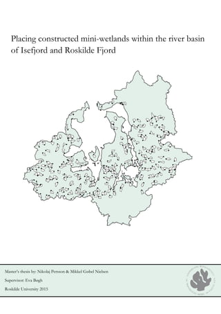
  • 8. 7 nitrogen reduction targets have been assigned to each of the coastal waters, which the river basins have been designated upon (Naturstyrelsen, 2014). The nitrogen reduction targets can be obliged by either general or specific measures selected from the CM. The general measures are implemented by the government, while the specific measures are implemented by the municipals (Naturstyrelsen, 2011). It is a requisite, that measures both general and specific are not only selected based on environmental effects, but also their cost-effectiveness. The cost- effectiveness is a pivotal part of the WFD, hence it is a requirement, according to the WFD article 11 and appendix 3 b, that the specified goals are realized at the lowest possible cost (Eriksen et al., 2014). In Denmark the general cost-effectiveness has been calculated for each measure and presented in the CM, this however is not in compliance with the recipient oriented approach called for by the WFD. It is not immediately meaningful to assess the general cost-effectiveness of each type of measure, as the actual cost-effectiveness depends on the individual locality in question (ibid.). The river basin of Isefjord and Roskilde Fjord is sited in the northern part of Zealand and affects 20 municipals. The total area is 1952 km2 and discharges to Isefjord and Roskilde Fjord. The river basin is dominated by agricultural activity, which covers 62% of the area and contributes to 77% of the waterborne nitrogen entering the fjords. As a consequence of an unnatural high nitrogen supply there has been registered an increase in phytoplankton growth and annual macro algae in both fjords. This in turn has led to a recession in eelgrass and benthic fauna. Today 74% of the total fjord area is classified as having a moderate ecological status and 26% as having poor ecological status. At present estimated 1668 tonN/yr discharges to both Isefjord and Roskilde Fjord. It has been estimated by the Danish Nature Agency that, to achieve good ecological status within both fjords, discharge must be reduced to a total of 1400 tonN/yr, hence a reduction of 268 tonN/yr is required (Naturstyrelsen, 2014). In connection to the development and implementation of the 2. generation RBMP, The Ministry of the Environment and Food and the Ministry of Climate, Energy and Building in 2014 forwarded a request for an updated and extended version of the CM, with increased focus on the integration of novel nitrogen reducing measures. The Danish Centre for Food and Agriculture has therefore devised an updated version of the CM. One of the novel nitrogen reducing measures is constructed mini-wetlands (CMW) (Eriksen et al., 2014). A CMW is a small sized measure specifically designed to target nitrogen transport derived from head-drains and ditches. The CMWs are fairly untested in relation to nitrogen removal from agricultural drain water, but have long shown good results in wastewater treatment on a global scale (Kadlec & Wallace, 2009). Even though it is commonly recognized, that CMWs work as effective measures in relation to wastewater treatment, recently undertaken Danish experiments, facilitated by the SupremeTech research project and Orbicon, have demonstrated that the CMWs also possess great potential as a measure to remove nitrogen derived from agricultural tile drains (Eriksen et al., 2014). Based on the experience derived from the SupremeTech research project and Orbicon, it has been proposed that the location associated to the placement of the CMW must meet certain conditions in order for the CMW to remove high amounts of nitrogen thereby being a cost-effective measure. The most essential challenges lies within finding the critical areas affected by both high nitrogen leaching and drainage, while at the same time ensuring a wetland to watershed ratio facilitating high hydraulic retention time (ibid.).
  • 9. 8 The focus of this thesis concerns the implementation potential of CMWs on a river basin level. The river basin of Isefjord and Roskilde Fjord is selected as case, to test where and how CMWs can be implemented to comply with the nitrogen reduction target of 268 tonN/yr and still being a cost-effective measure. The abovementioned results in the following problem formulation: 1.1. Problem formulation Where and how can constructed mini-wetlands be placed in order to work as a cost-effective measure complying with the nitrogen reduction target of Isefjord and Roskilde Fjord? 1.2. Working questions To help us structure the answering of the problem formulation following working questions have been devised.  Where can constructed mini-wetlands be placed in order to facilitate nitrogen removal?  Which of the potential constructed mini-wetlands can be considered cost-effective?  With how many ton of nitrogen can the cost-effective potential constructed mini-wetlands reduce the nitrogen load to Isefjord and Roskilde Fjord a year?  How can the potential constructed mini-wetlands implementation potential be assessed? 1.3. Delimitation  This thesis only assesses the potential of implementing constructed mini-wetlands related to the removal of nitrogen, derived from agriculture. Phosphorous could also have been screened for, as it can be a limiting nutrient in phytoplankton growth thereby affecting risk of hypoxia within coastal waters.  The screening model does not take into consideration areas affected by regulation as Natura2000 or The Nitrate Directive etc. when screening for potential placements for constructed mini- wetlands. Neither does the screening model include the nitrogen removal effect related to groundwater.  Different types of constructed mini-wetlands exist. The screening model in this thesis is developed around Orbicon’s concept of a constructed mini-wetland, which is a constructed mini- wetland with horizontal subsurface-flow (HSSF).
  • 10. 9 2. Theory Following chapter clarifies theory, which establishes the foundation of answering the problem formulation. The chapter is initiated by a presentation of the nitrogen cycle including nitrogen transfers, processes, chemical forms and effects. Hereafter the physical, chemical and hydrological aspects of nitrogen movement in agricultural soils will be presented. This is followed by a presentation of watershed hydrology and the removal of nitrogen from field to fjord. Furthermore an economical subsection is added to accommodate the problem formulations focus on cost-effectiveness of CMWs. In the final part of the theory chapter natural and constructed wetlands are presented, here among Orbicon’s version of a CMW and its physical and economical key-figures. 2.1. The Nitrogen Cycle Nitrogen is required by all organisms in different processes supporting the basic building blocks of life, such as amino acids, nucleic acids and chlorophylls. Nitrogen, phosphorus and potassium are the three primary macronutrients required in plant growth. Nitrogen is often the most limiting nutrient affecting the regulation of primary production. Within ecosystems there exists a wide range of nitrogen compounds in different forms. Between the most oxidized and reduced compounds nitrogen has an electron difference of eight, descending from ammonium (NH4 + ) to nitrate (NO3 - ). Ammonium and nitrate are the two forms, which are available for plant uptake (Smith & Smith, 2008). Nitrogen can be found in reservoirs as the atmosphere, biosphere, oceans and geological as both organic and inorganic nitrogen (Ward, 2012). Organic nitrogen includes a range of proteins and urea considered an animal waste product used as fertilizer. Inorganic nitrogen is the most common form and includes: dinitrogen (N2), ammonium (NH4 + ), ammonia (NH3), nitrite (NO2 - ), nitrate (NO3 - ), nitric oxide (NO) and nitrous oxide (N2O) (Vymazal, 2006). In its cycle, nitrogen is converted between several of chemical forms in a chain of processes. These processes can either take place in anaerobic or aerobic environments. Some processes are mediated by organisms obligate to oxygen, while others are facultative. Facultative organisms thrive in both anaerobic and aerobic environments, while obligate organisms are dedicated to only one (Prescott et al., 1996). The nitrogen cycle begins with the conversion of atmospheric nitrogen into ammonium. This process can take place in aerobic as well as anaerobic environments (nitrogen fixation). The process of nitrogen fixation is mediated by bacteria transforming ammonium into a biologically available form. Most nitrogen fixating bacteria exist in a symbiotic relationship with plants. Once the plants die they undergo decomposition, a process where the nitrogen containing parts will be degraded into inorganic nitrogen facilitated by microorganisms (ammonification). In the process of decomposition, ammonium is released into the environment as a waste product. The transformation of organic nitrogen into ammonium can occur in both aerobic and anaerobic conditions. The released ammonium is either re-assimilated by microorganisms or plants (ammonium assimilation) or oxidized by chemoautotrophic bacteria in the aerobic part of the environment (nitrification).
  • 11. 10 The oxidized forms of nitrogen are either assimilated by microorganisms and plants (nitrate assimilation) or reduced by facultative anaerobic bacteria under anaerobic conditions (denitrification). The reduction of nitrate by microbial processes ultimately produces dinitrogen as a waste product. Production of dinitrogen completes the nitrogen cycle returning it back to the atmosphere. See fig. 1 for a schematic review of the nitrogen cycle and nitrogen transformation (Smith & Smith, 2008; Reddy & DeLaune, 2008). Figure 1: Shows the nitrogen cycle and the transformations of nitrogen between the aerobic and anaerobic environment (Bernard, 2010). Aerobic part of the nitrogen cycle The majority of the processes in the nitrogen cycle occur in aerobic environments, the processes are nitrogen fixation, ammonification, nitrogen assimilation and nitrification. Nitrogen fixation takes place in both the anaerobic and the aerobic environment (Reddy & DeLaune, 2008). Nitrogen fixation Nitrogen fixation is defined by the ability to fix atmospheric nitrogen and convert it into a biologically available form. Nitrogen fixating organisms, usually in symbiotic or mutualistic relationship with plants, provide the plants with ammonia in exchange for carbohydrates (Vymazal, 2006; Canfield et al., 2005; Gurevitch et al., 2006). Studies have shown, that nitrogen fixation occurs in greater amounts in anaerobic soils than aerobic, where it is the other way around when the soils are flooded. The input to the biosphere by nitrogen fixation is balanced by the output of denitrification. The input from nitrogen fixation along with other sources contributes with 92×106 ton of nitrogen to the biosphere a year. In non-oceanic environments 78% of nitrogen input derives from biological fixation, while 20% and 2% derives from industrial fixation and lightning respectively. Each year approximately 9.78% of the input is fixated into the biosphere. The remaining 90.22% is lost from the biosphere to the atmosphere mainly through denitrification. The process of fixing nitrogen into a biologically useful form is therefore important, as it is needed to replace lost nitrogen (Reddy & DeLaune, 2008).
  • 12. 11 Nitrogen assimilation Assimilation of nitrogen is the formation of inorganic nitrogen to biologically available organic compounds. When nitrogen is assimilated by plants, it becomes immobilized and does not circulate further until mineralized. Plants lagging the ability to fixate nitrogen depend on their ability to assimilate available forms of nitrogen. Inorganic nitrogen assimilated by plants is quickly metabolized into organic nitrogen containing compounds (Reddy & DeLaune, 2008). Plants need nitrogen in large amounts to grow, reproduce and perform photosynthesis. The two major forms of nitrogen taken up by plants are ammonium and nitrate. Ammonium is taken up by the roots and transported to the shoots or incorporated directly into organic compounds (Gurevitch et al., 2006). When ammonium is low, nitrate can be taken up by assimilatory nitrate reduction to ammonium (ANRA). ANRA is a process where ammonium is produced by the reduction of nitrate. ANRA generally occurs in aerobic soil environments, where nitrate is most stable. (ibid.). Ammonification Ammonification is a process where heterotrophic microorganisms release ammonium by decomposing organic matter. The process of this release is called deamination and is an enzymatic process that removes nitrogen from organic matter eventually releasing it as ammonium (Canfield et al., 2005). The released ammonium may either become mobilized and act as an excess source of nitrogen or immobilized and be taken up and incorporated into new biomass. Ammonification occurs primarily under aerobic conditions, but can also take place under anaerobic conditions however deamination is less efficient under anaerobic conditions (Gurevitch et al., 2006). Nitrification Nitrification is defined by the process of oxidizing ammonium to nitrite and further into nitrate. The process covers the most reduced and oxidized forms of nitrogen and provides denitrification with oxidized nitrogen (Gurevitch et al., 2006). A number of bacteria perform nitrification, the most common group is chemolithoautotrophic. Chemolithoautotrophic organisms have an obligate aerobic metabolism, but research has shown that an anaerobic metabolism also can occur (Canfield et al., 2005). The two most important genera of nitrifying bacteria are Nitrosomonas and Nitrobacter, these organisms are physiologically unrelated but work in close relationship. The first reaction of oxidizing ammoniumto nitrite is executed by Nitrosomonas. The second reaction is the oxidation of nitrite to nitrate and is performed by Nitrobacter (ibid.). The two genera of bacteria are under normal circumstances found together in soils and sediments, where the close relationship between the two groups of bacteria prevents nitrite from accumulating, which is why nitrate is more common in these environments (ibid.).
  • 13. 12 Anaerobic part of the nitrogen cycle Oxidized forms of nitrogen produced by nitrification, which is not assimilated by microorganisms or plants, diffuse downward into the anaerobic zone. This diffusion is facilitated by a difference in concentration gradient. Under anaerobic conditions nitrogen is reduced by facultative anaerobic bacteria utilizing nitrate as an electron acceptor to gain energy by oxidizing organic matter. The reduction of nitrate it dominated by dissimilatory nitrate reduction processes (Reddy & DeLaune, 2008; Canfield et al., 2005). In general there are three dissimilatory processes using nitrogen oxides as electron acceptors by the reduction of nitrate: Dissimilatory nitrate reduction to ammonium (DNRA), anaerobic ammonium oxidation (anammox) and denitrification (Canfield et al., 2005). DNRA DNRA is mediated by obligate anaerobic bacteria and tends to take place in soils which are permanently under anaerobic conditions. The process requires a high availability of electrons and a low redox potential to execute the process to completion (Reddy & DeLaune, 2008). The complete nitrate ammonification proceeds in two steps: NO3 -  NO2 - NO2 -  NH4 + Equation 1: Shows the DNRA in two steps. First nitrate is converted to nitrite and second nitrite is converted to ammonium. Anammox Anammox, is the process of oxidizing ammonium to dinitrogenusing nitrate or nitrite as an electron acceptor. The idea of anammox occurred nearly four decades ago, though it is just within recent years, the bacteria mediating the process has been isolated and the process documented. The only known bacteria mediating the process of anammox is chemolithoautotrophs, the reaction proceeds as follows: 5NH4 + + 3NO3 -  4N2 + 9 H2O + 2H+ or NH4 + + NO2 -  N2 + 2H2O Equation 2: Shows the anammox process producing dinitrogen by the oxidation of ammonium using nitrate or nitrite as as electron acceptors. The metabolic pathway of anammox is not yet fully understood, but the process may contribute substantially to the production of dinitrogen in nitrate rich environments (Canfield et al., 2005).
  • 14. 13 Denitrification Denitrification is a process where nitrate and nitrite is converted to gaseous end products and ultimately into dinitrogen. The process is mediated by facultative anaerobic bacteria, such as Paracoccus denitrificans, utilizing nitrate as an electron acceptor in a chain of respiratory reduction steps to gain energy (Canfield et al., 2008). There are several respiratory reduction steps in the transformation of nitrate to dinitrogen. The respiratory reductions steps of nitrogen electron acceptors, are in preferred order of most to least thermodynamically favorable: NO3 -  NO2 -  NO  N2O  N2. Production of dinitrogen can be regarded as a completion of the nitrogen cycle by emitting the nitrogen back to the atmosphere, turning denitrification into a major sink for nitrogen (Vyzamal, 2006). The reduction nitrate to dinitrogen can be segregated into four steps or modules, each executed by its own enzyme catalyzing the process. The first step is executed by the enzyme nitrate reductase, a membrane bound enzyme that produce nitrite and hydroxide. The nitrite is subsequently reduced by nitrite reductase an enzyme located inside the cell, producing nitrogen monoxide and water. This enzyme may under strong reduced conditions and at high pH produce nitrous oxide. Subsequently nitrogen monoxide is reduced to nitrous oxide by the enzyme nitric-oxide reductase, which is also located inside the cell of the bacteria. The last step converts nitrous oxide to dinitrogen, the process is executed by nitrous-oxide reductase. Nitrous oxide, as an electron acceptor, provides the denitrifying bacteria with enough energy that bacteria can grow solely on the expense of this reaction (ibid.). Having the enzyme converting nitrous oxide to dinitrogen inside the cell, reduces the chance to emit the greenhouse gas nitrous oxide to the surrounding environment and atmosphere (Canfield et al., 2008.). Environmental deficiency of the essential metals iron (Fe), copper (Cu) and molybdenum (Mo) can also block the biosynthesis of one or several of these enzymes, which potential could result in a high emission of nitrous oxide (ibid.). The emission of nitrous oxide can have a negative effect on global warming as nitrous oxide is 298 times more efficient to trap heat within the atmosphere compared to CO2 (EPA, 2013). The process of denitrification depends on how the different modular respiratory processes work together. As Canfield et al. (2008) points out: “Complete denitrification can only be viewed as the modular assemblage of four partly independent respirator processes. Complete denitrification is achieved only when all modules are activated simultaneously.”
  • 15. 14 2.2. Nitrogen movement in agricultural soils In an agroecosystem the importance of decomposition is less significant, compared to a natural ecosystem. This is because crops including their nutrients are harvested and removed permanently from the field, thereby hindering the natural decomposition of organic matter and release of nutrients back to the soil (Smith & Smith, 2012). As a consequence organic and mineral fertilizer has to be added to maintain a satisfying level of nutrients to support crop production (ibid.). In the late 1800s there came an increased demand for food, as the world population increased. This demand was followed by an increased demand of fertilizer and especially nitrogen. In 1913 the first chemical plant succeeded to synthesize ammonia by fixing atmospheric dinitrogen. The process of use became known as the Haber-Bosch process (ibid.). During the 20th century the Haber-Bosch process was improved and came to play a huge part in the Green Revolution. Today the Haber-Bosch process has provided the agricultural sector with an unlimited source of nitrogen, which has caused an increased nitrate leaching from the fields to the marine environments (ibid.). The interactions between the material and hydrological properties of a soil, affects the soils inclination to repulse and leach nitrogen into the marine environments. Soil Properties Soil texture The chemical and physical properties of a soil derive to a high degree from the distribution of grain- minerals within the soil. Grain-minerals are classified by size (See tab. 1). The grain-size distribution is determined from a soil texture triangle (Dingman, 2004). The soil texture triangle weighs the distribution of clay, silt and sand by percentage, thereby determining the grain-size distribution of the soil. Based on the grain-size distribution, the soils are classified by texture also known as texture-classes (See fig. 2). Clay content of a soil controls, to a large degree, the soils ability to leach nitrate and adsorb ammonium between the soil water solution and the grain-minerals (Moore, 2001). Grain-minerals Unit (mm) Sand 0.05 - 2 - Very coarse 1 – 2 - Coarse 0.5 – 1 - Medium 0.25 - 0.5 - Fine 0.1 - 0.25 - Very fine 0.05 - 0.1 Silt 0.002 - 0.05 Clay < 0.002 Figure 2: Shows the soil texture triangle and the proportion of clay, silt and sand shown as a percent. By weighing the distribution of clay, silt and sand, 12 texture-classes can be distinguished (Bøgh, 2012). Table 1: Shows the three most common grain- minerals: sand, silt and clay and their respective grain-size.
  • 16. 15 Pore-size and capillary action Pore-size is a consequence of the grain-mineral size. Hence, pores are bigger in soil textures comprised by sand and silt compared to clay. Pores are categorized as micropores, mediumpores and macropores based on the size in space between grain-minerals. Sandy soils have few but wide pores, caused by the rotund shape of sand-minerals. Clay soils are composed by small disc-shaped clay-minerals, causing micropores to occur and few macropores (See fig. 3) (Dingman, 2004). Sandy soils have high drainage as a function of the high amount of macropores between grain-minerals. Conversely water is held more tightly within the micro and mediumpores, provided by clay and silt- minerals. This is a result of the capillary action retaining or moving water in an upward direction. The upward movement of water in a soil is known as capillary rise. A capillary rise will happen when the waters cohesive intermolecular forces are exceeded by the intermolecular adhesive forces between water and a solid object. Capillary rise is expressed as upward movement through the soil and increases inversely with pore space. Hence, capillary rise is high in fine textured soils like clay and silt and low in sandy soils (See fig. 4) (CTAHR, 2015). Figure 4: Shows the capillary rise as a consequence of soil- pore size. Narrower tubes have a higher capillary rise compared to wide tubes. Coarse sand can transport water in a height between 20-50 cm, while clay can transport water in a height above 80 cm. (CTAHR, 2015). Figure 3: Shows the grain-minerals: sand, silt and clay including the composition of pore- size and their ability to withhold water from leaching in a soil-profile. A sandy soil has high amount of macropores and can therefore withhold less water. A soil composed of silt has an even distribution of both macro and micropores and is therefore better to withhold water from leaching compared to a sandy soil. Clay soils have high amounts of micropores and withholds large amounts of water from leaching (CTAHR, 2015)
  • 17. 16 Hydrologic soil horizons A hydrological soil profile consists of a: root zone, intermediate zone, tension-saturated zone and groundwater zone(See fig. 5). The unsaturated zone is a zone of negative water pressure (ψ < 0) extending from the soil surface to groundwater table. The root zone extends from the upper soil surface to a lower boundary, defined by the depth, in which plant roots are able to extract water. Water entering the root zone originates from infiltration and leaves as either drainage or evapotranspiration. Water entering the intermediate zone originates from the root zone and leave as drainage. The interface between the unsaturated zone and saturated zone is the tension-saturated zone, in which pore spaces function as capillary tubes, and surface-tension forces, draws up water, creating a nearly saturated environment. The groundwater zone is saturated and has a positive water pressure (ψ > 0) (Dingman, 2004) Figure 5: Shows the hydrological soil profiles extending from groundwater to the root zone. From the root zone being an unsaturated environment to the saturated groundwater, there can be drawn a water pressure profile. The profile indicates the water pressure and water saturation of the soil (Dingman, 2004).
  • 18. 17 Nitrate-leaching Leaching is the process whereby dissolved debris, minerals and ions in solution are carried downward by water in a soil profile (Lehmann & Schroth, 2003). Nitrate leaching is the result of nitrate becoming unavailable for plant uptake, by leaching below the root zone. The amount of nitrate leaving the root zone is controlled primarily by two factors: the nitrate concentration in soil water and soil drainage (Gustafson, 2012). Rates of nitrate leaching are temporally distributed. Most nitrate leaching occurs in temperate regions in winter months, where precipitation and concentrations of nitrate is high (Cameron & Di, 2002). Soil drainage Water within the unsaturated zone has a negative water pressure or tension. Tension increases as water content decrease (See fig. 6). The relationship between water content and tension is given by the soil moisture retention curve. In the soil moisture retention curve tension is expressed in a pF scale corresponding to the negative base 10 logarithm of the water pressure. For a fully saturated soil pF equals 0 and increases by decreasing water content (Bøgh, 2014). When pF ≤ 2 drainage occurs from the root zone. Conversely water is withheld from drainage when field capacity (FC) is reached at pF ≥ 2 (See fig. 6). Because plants cannot exert tension above pF 4.2, transpiration ceases around this limit and plants begin to wilt, this is the wilting point (WP). The difference between FC and WP is the available water content (See fig. 6). Soil water is hydroscopic when tension exceeds pF 4.5, which results in water being absorbed from the air (Dingman, 2004). Figure 6: Shows three curves for sand, loam and clay depicting the relationship between water content and water pressure (tension) given in a pF scale. As can be observed clay soils are able to withhold more water (48%) compared to loamy (30%) and sandy (8%) soils at F.C. (Lajos, 2015)
  • 19. 18 Clay mineral ammonium fixation Nitrogen exists in many forms within the soil environment, but only nitrate leaches in appreciable amounts from the root zone due to its negative charge. On the other hand, the positive charged ammonium ion, adsorbs to the soil surface and is thereby withheld from leaching (Cameron & Di, 2002). Soils are able to adsorb anions and cations to its surface. In temperate regions most soils are dominated by cation exchange, caused by the negatively charged colloids (crystalline silicate clay and humus) (Cameron & Di, 2002). Silicate clay particles are negatively charged colloids, given they have been subjected to an isomorphous substitution of silica (Si4 + ) by aluminum (Al3 + ). Because aluminum has a lower valence than silica, the net charge becomes negative (See equ. 3). Equation 3: Shows the substitution of silica with aluminum turning the colloid negative. Due to electrostatic forces the negative colloids attract and adsorb ammonium, this process is called clay mineral ammonium fixation. The lyotropic series divide the most common cations in soil, based on the bonding strength between the cation and the colloid. The bonding strength is a result of the size and positive charge of the cation (Brereton, 2014). The cations are in a dynamic equilibrium, where smaller and more positively charged ions, in soil solution exchange with cations already adsorbed by clay and humus. The capacity of the soil to withhold cations is determined by the cation exchange capacity (CEC). The CEC changes as a function of colloid composition (clay and humus) and pH. In general CEC is high when clay or humus content is high and pH is neutral to alkaline (Brereton, 2014). Humus is an organic substance consisting of mainly carbon and hydrogen. Humus carries a negative charge due to the dissociation of mainly phenol, hydroxyl and carboxyl groups adding H+ to the soil solution and leaving O- in the humus complex (See fig. 7). The negative charge of clay and humus prevents ammonium from leaching. Because nitrate is a negatively charged ion, the same effect that attracts ammonium in colloids repulses nitrate. Therefore nitrate is left as a free ion exposed to leaching (Ketterings, 2007).   442 SiAlOOSi   NaNHKMgCaHAl 4 223 Figure 7: Shows a humus complex and the dissociated groups of phenol, hydroxyl and carboxyl creating a negatively charged colloid (Brereton, 2014).
  • 20. 19 2.3. Watershed hydrology Watershed definition A watershed is a defined biophysical system based on topographic boundaries delineating the surface area of a landscape where water, nutrients, sediments and chemicals drain to a common body of water. The water body can be a lake, estuary, reservoir, ocean, wetland or any point in a stream. The delineation of a watershed follows the topography of the surface area. Hence ridges and hills often characterize the drainage divide, where two watersheds separate (See fig. 8) (Maiden, 2000). Figure 8: Shows two watersheds defined by a drainage divide (Study blue, 2014). The hydrological cycle Water is in an everlasting circulation driven by the forces of radiation emitted from the sun and gravity. The circulation of water on earth is known as the hydrological cycle. The hydrological cycle consists of a numerous of hydrological processes and pathways. These processes and pathways constitute the movement of water from the earth’s surface to the atmosphere and back again. Within the hydrological cycle water is neither gained nor lost, only the amount of water between the different reservoirs changes over time. The hydrological cycle is driven by radiation emitted from the sun heating the atmosphere and making energy available for evaporation. The vaporized water is carried by winds and precipitates as rain or snow, when climatic conditions favor condensation (Brooks, 2013). The water balance The water balance is a simple and quantified interpretation of the hydrological cycle. The water balance builds on the principle of the conservation of mass law. The principle dictates that input to a watershed equals output and change in storage in a closed system. This means, if input exceeds output over time, there must be an increase in storage and vice versa. The conservation of mass law is applicable to the water balance equation (See equ. 4) (ibid.).
  • 21. 20 Equation 4: Where P = precipitation (mm), GWI = groundwater flow input (mm), Q = stream flow (mm), ET = evapotranspiration (mm), GWo = groundwater outflow (mm) and ΔS = change in storage (mm). In the water balance equation, the inputs to the watershed are P and GWI where Q, ET and GWo are outputs. Note that drainage through drains is categorized as groundwater, as drains are considered having a saturated environment. Often the water balance is simplified, since it is assumed that ΔS, GWI and GWo do not change over time, if no significant, climatic, geologic or anthropogenic changes have taken place within the watershed. Hence the water balance can be simplified to equation 5 (Brooks, 2013). Equation 5: Shows the simplified water balance where P is precipitation, Q is stream flow, ET evapotranspiration and ΔS is change in storage. Soil water transfer processes Interception Interception is the direct loss of water through evaporation from the plant surface. Water that is not lost through interception reaches soil and infiltrates the ground (Brooks, 2013). Infiltration Infiltration is a result of gravity and the capillary action within the soil. If the intensity of precipitation exceeds infiltration, overland flow will occur. If overland flow concentrates in depressions or gullies, the water will move from a sheet flow to a channelized flow. Infiltrated water moves vertically through the ground, if field capacity is exceeded (ibid.). Percolation The downward drainage of water is known as percolation. If percolation of water reaches an impermeable soil stratum like clay or solid bedrock, water will move in a horizontal direction along the layer as interflow. Interflow often discharge to surface water. Water, which is not draining as interflow percolates downwards and becomes groundwater (ibid.). Evapotranspiration Evapotranspiration can be partitioned into: interception, evaporation and transpiration. Interception is the evaporation of water from the surface of vegetation or dead organic matter back to the atmosphere. Evaporation is the loss of water from any surface area and body of water, as well as the upper layer of the soil to the atmosphere. Transpiration is evaporation initiated by the absorption of soil water from plant roots. The water is transported from the roots through xylem and released as vapor through leafs to the atmosphere (ibid.). SGWETQGWP oii  SETQP 
  • 22. 21 2.4. Denitrification from field to fjord Nitrate leaching from agricultural areas moves to surface water as horizontal flow. Horizontal flow is water moving in a lateral direction as either overland flow interflow or groundwater flow ultimately discharging to coastal water (Hinsby, 2014). The resulting quantities of nitrate draining to the coastal ecosystem, depends on the pathways and processes nitrate undergoes from field to fjord. If nitrate containing water interferes with an anaerobic environment, the nitrate can degas as atmospheric nitrogen (See chapter 2.1.2). Anaerobic environments are mainly present below the nitrate-front and in stream, lake and wetland sediments. Anaerobic environments can also temporally occur by sudden soil saturation or in areas of high microbial activity. A conceptual movement of nitrate from field to fjord is depicted in fig. 9. The nitrate-front The division between aerobic and anaerobic environments within a soil-profile is known as the nitrate- front. The nitrate-front is the area within the soil-profile, where oxygen levels are low enough to facilitate microbial respiration, by the use of nitrate instead of oxygen. The nitrate-front can be difficult to determine, but a general distinguishment can be made from the soil color. I.e. soils having yellow to yellow-grey colors are said to be within an aerobic environment with high nitrate levels. Conversely, soils with grey and black colors are associated with an anaerobic environment and low levels of nitrate (Ernsten, 2014). Figure 9: Shows the movement of nitrate from field to coastal water including the nitrate-front (redox boundary) (Dahl & Hinsby, 2013)
  • 23. 22 Denitrification within the aerobic unsaturated zone Nitrate reduction can also occur in anaerobic environments within the general aerobic unsaturated zone. Nitrate reduction in the unsaturated zone is related to the high amount of organic matter which is oxidized through microbial respiration, creating a local anaerobic environment. Nitrate reduction within the unsaturated zone is limited to depths, where organic matter is regularly supplied by plant cover, which is 3-5 m below surface (Mossin et al., 2004). Groundwater Groundwater is stored in aquifers made up by unconsolidated materials or water-bearing bedrock. The aquifer can be classified as either primary or secondary. A primary aquifer is sited at greater depths than the secondary, often between 30-300 meters below surface (Thuesen, 2014). Primary aquifers are often located where gravel, sand and chalk deposits are present and consist of one or more linked aquifers. A secondary aquifer is sited closer to the surface in clay pockets filled with water conducting sand (Thuesen, 2014). A secondary aquifer is limited in size and present above the water table defined by the primary aquifer. Under natural conditions groundwater discharges to surface waters as lakes, streams and wetlands, which eventually discharges to coastal ecosystems. Groundwater can also enter surface water through springs or brooks, if the recipient is sited lower than the water table (Winter, 1998). The faith of nitrate in groundwater depends on the oxygen level within the soil. Secondary aquifers which are close to the surface are generally high in oxygen compared to primary aquifers. Within secondary aquifers nitrate is present, while primary aquifers sited at greater depths are able to reduce the nitrate. The process of denitrification within anaerobic groundwater is highly dependent on the amount and composition of available soil reducing compounds. Important reducing compounds are organic carbon (C), pyrite (FeS2), Ferro iron (Fe2+ ) and methane (CH4). These compounds are generally available within the anaerobic soil environment, but are quickly oxidized by microbial processes within the aerobic environment (Ernsten, 2014). Tile drainage The primary reason for tile drainage is to increase plant productivity by either lower the water table or increase the rate of percolation to groundwater (Nielsen, 2015). Modern day tile drains are perforated plastic tubes allowing water to enter through small perforations. In a loamy soil tile drains are buried in an average depth of 1 m below surface, within an average distance of 15 m (Wright, 2001). Tile drains can be considered as small “highways” discharging nitrate rapidly to surface waters, preventing nitrate from becoming available for nitrate assimilation or denitrification. Tile drains are considered having a saturated but aerobic environment because of their relative proximity to the surface, hence no nitrate reduction is presumed within tile drains (Refsgaard, 2014). This situation changes, if tile drains pass through an anaerobic environment i.e. a lowland. A tile drainage system consists of side-drains (80 mm) and head-drains (90-210 mm) (Nielsen, 2015). The tile drains can be assembled in different system layouts as depicted in fig. 11. Whether choosing one from the other depends on the field topography and the location of the outlet. Common for the system layouts are that side-drains drain to a head-drain, which usually drains into a ditch or stream (ibid.). A parallel system layout which is very common is depicted in figure 10.
  • 24. 23 Stream Streams are characterized by having a uni-directional flow closely dependent on the surrounding watershed. Stream discharge is a result of net precipitation available as runoff from overland flow, interflow and groundwater (baseflow). Water entering a stream as interflow and overland flow is fast running and predominant in periods of high net precipitation. In loamy watersheds, interflow has a high impact on stream discharge, compared to a sandy watershed. This is caused by a decreased by-pass flow, caused by the fine-grained loamy soil (Winter, 1998). Baseflow is a continuous inflow of water through the streambed. Baseflow can enter a stream as a spring, if the water table is above the stream surface. Conversely, surface water can seep to groundwater, if the water table is sited lower than stream surface (ibid.). Nitrogen retention in stream environment Nitrogen removal in a stream environment is mainly facilitated by denitrification. Denitrification is only active in the anaerobic parts of the sediment or in the innermost layer of biofilms. Nitrate becomes part of the denitrification process, as either nitrate diffuses directly from the water column to the sediment or is produced by nitrification within the aerobic layers of the sediment, the latter process is known as coupled nitrate-denitrification (Allan & Castillo, 2007). Nitrate diffuses directly from the water column into sediment as a consequence of high nitrate concentrations in the water column and low concentrations in sediment. The coupled nitrification-denitrification sequence is regulated by upward diffusion of ammonium leached from particulate organic matter within the anaerobic sediment into aerobic sediment. In the aerobic sediment the ammonium undergoes nitrification and nitrate diffuses downwards into the anaerobic layer and denitrifies (ibid.). Nitrogen assimilation facilitated by macrophytes and algae, is an important part of the nitrogen retention within streams. Nitrogen assimilated by macrophytes is only momentarily retained in either living tissue, decomposing- and microbial biomass, or immobilized as particulate organic matter in sediment (ibid.). Figure 11: Shows four different system layouts commonly used for tile drainage (ONTARIO, 2015). Figure 10: Shows a parallel system layout on a field-scale. It can be seen that side-drains drains to a head-drain subsequently discharging to an open ditch (ONTARIO, 2015).
  • 25. 24 Lake A lake is a lentic ecosystem capable of removing nitrogen from the aquatic environment through denitrification and permanent burial of organic matter into sediment. The primary source of nitrogen within a lake derives as runoff from overlandflow, interflow and baseflow and nitrogen fixation by cyanobacteria (Banta, 2014). Input of carbon is mainly autochthonous, while nitrogen input is allochthonous (ibid.). The denitrification in the anaerobic sediment is fed by nitrate from the aerobic sediment or the water column (Sybil, 1998). The hydraulic retention time is an important lake feature affecting nitrogen removal. Rates of denitrification increase by increased hydraulic retention time. Equation 6: Windolf et al. (1996) established an empirical relationship between lake nitrogen concentration (Nlake), hydraulic retention time (tw) and nitrogen inflow concentration (Ninput). Depth is another important lake feature influencing the nitrogen removal. When lake mean depth is above 5-7 m a thermocline can arise during warm periods creating an impermeable layer between hot less dense water at the top (epilimnion) and cold dense water at the bottom (hypolimnion) (Wetzel, 2001). The thermocline can prevent nitrogen from entering the sediment and thereby become subjected to denitrification or permanent burial. In addition increasing depth decreases the chance for a given water volume to get in contact with sediment. Consequently deep lakes are less able to remove nitrogen compared to shallow lakes (Søndergaard, 2007). Shallow lake systems Shallow lakes are lakes where macrophytes are able to thrive throughout the whole lake, and a thermocline is not present. In general lakes are said to be shallow when the mean depth is below 5-7 m (Scheffer, 2004). Shallow lake systems are effective in removing nitrogen from the aquatic environment due to a combination of continuous mixing of nitrogen rich water into sediment, and a high contact surface between water and sediment (ibid.). From empirical studies it has been observed, that shallow lakes having a hydraulic retention time exceeding a month can remove more than 50% of the nitrogen input to the lake. A relationship between hydraulic retention time and nitrogen retention for shallow lake systems can be seen from fig. 12 (ibid.). Figure 12: Shows the mean nitrogen retention (%) as a variable of the hydraulic retention time based on four years of measurement for 16 shallow Danish lakes (Scheffer, 2004) tw N N input lake   32.0
  • 26. 25 Fjord A fjord is a semi-enclosed part of the ocean surround by land on three sites (See fig. 13). The ecosystem is characterized as a mixing zone of freshwater and saltwater. A fjord is associated with a sill at its mouth, functioning as a threshold between brackish water and oceanic saline water (NIWA, 2015). Figure 13: Shows a conceptual presentation of a fjord, including the water movement of the less dense brackish water going outwards on top of the saline water moving on top of the sill in an inwards direction (Rekacewicz & Bournay, 2007). Nitrogen input to a fjord derives as: watershed runoff, atmospheric deposition, oceanic transport and nitrogen fixation. The primary nitrogen input supporting primary production within a fjord derives as nitrate, ammonium and dissolved organic nitrogen (Bowen, 2001). Nitrogen removal is primarily facilitated through dissimilatory nitrate reduction, with denitrification contributing to the primary removal and anammox being of less importance (See chapter 2.1.2.). A vast amount of the nitrogen is also lost permanent as burial within sediment (Voss, 2011). In general nitrogen input exceeds output, therefore the fjord is often perceived as a nitrogen filter to the ocean. The movement of water and nitrogen within a fjord is severely affected by a salt wedge (pycnocline). A pycnocline occurs as a consequence of less dense freshwater discharging from land, in an outward direction on top of the dense seawater moving from the ocean towards the coast (See fig. 14). These two opposing currents create a nutrient trap, where nitrogen settles at the bottom. The high ionic strength in saltwater drives the flocculation and sedimentation of organic matter in terrestrial freshwater, at the onset of the pycnocline (sediment accumulation). Combined nutrient trapping and sediment accumulation constitutes the turbidity maximum zone (See fig. 14). The turbidity maximum zone is a highly active zone of nitrogen transformation and removal, caused by high amounts of organic matter and nitrogen (ibid.). The denitrification process is highly dependent on the availability of organic matter, nitrate and retention time. Due to high primary production organic matter is often in excess, while nitrate becomes the limiting nutrient. This is especially the case, when hypoxic conditions occur, and nitrification is prohibited. As with lake systems the retention time plays a significant role in the process of denitrification. Increasing retention time increases the chance of nitrate to diffuse into anaerobic sediment and become subjected to denitrification. Fjord retention time is controlled by the exchange rates of water from inputs and tidal movement towards the ocean and the estuarine volume (ibid.).
  • 27. 26 Figure 14: Shows the outward movement of freshwater on top of oceanic saline water moving in an inward direction towards the fjord. The mixing waters create a pycnocline where a turbidity maximum zone occurs. In the sediment within the turbidity maximum zone, organic matter accumulates and supports the process of denitrification (Fischer, 1995). Hypoxia When oxygen levels are below 2 ml l -1 the water is said to be hypoxic (Voss, 2011). Hypoxia is favored when mainly two factors are present. First bottom water has to be prohibited from mixing with oxygen rich surface water. Second a considerable amount of organic matter needs to be available for oxidative bacterial respiration (See chapter 2.1.1.). The primary source of organic matter within a fjord derives from phytoplankton having a primary production limited by nitrogen. Excess nitrogen from terrestrial environments facilitates high primary production by phytoplankton, which in turn deprives the fjord water of oxygen. As nitrification depends on oxygen being present, hypoxia can prohibit this process. This in turn facilitates an accumulation of ammonium, causing an additional oxygen depletion. (ibid.).
  • 28. 27 2.5. Cost-effectiveness analysis A cost-effectiveness analysis (CEA) is an economic method used to compare the cost and benefits associated to different projects. The cost effectiveness is presented as a cost-effectiveness ratio (CER), where E is an environmental unit i.e. kg nitrogen removed and C is the cost in monetary units (See equ. 7) (Pearce, 2006). Equation 7: Where CER is cost-effectiveness ratio, C is cost and E is the environmental unit. The CER can be used to rank different projects and make decision makers capable of selecting the project with the highest effectiveness compared to the cost. In most CEA’s, projects are ranked based solely on their cost (AWWA, 2007). Annualizing the costs The goal of the CEA is to rank projects from another based on their CER. The CER is a product of the annualized costs grouped into capital expenditures (CAPEX) and operational expenditures (OPEX) divided by the annual benefit (ibid.). CAPEX A cost is considered as a capital expenditure, when the asset purchased is contributing to the project throughout its lifetime. Capital expenditures often occur early in the projects lifetime. In order to annualize the capital expenditure a capital recovery factor (CRF) has to be included. The CRF is calculated from equ. 8 (ibid.). ))1/1/(( n rrCRF  Equation 8: Where CRF is the capital recovery factor, r is the interest rate and n is the lifetime of the project The capital recovery factor is a way of calculating the loss of opportunity as an annuity (Khatib, 2003). The principle is grounded in the alternative investment, i.e. the benefits that could have been earned, had the invested money been put into its next best use. The next best use is normally putting the money into risk free assets such as government bonds and earn interest, hence the use of an interest rate. Both the interest rate and the lifespan of the project significantly affect the cost-effectiveness of the respective project. To find the annualized capital cost the CRF is multiplied by the capital expenditure (ibid.) E C CER 
  • 29. 28 OPEX Operation and maintenance expenditures also known as OPEX, are costs associated to operate and maintain a project on a daily basis (AWWA, 2007). These costs are normally annualized and include wages, rents, small reinvestments, insurance costs, employee travel etc. (Schmidt, 2015). OPEX and CAPEX are added to find the annualized cost of the project. When the annualized cost of the project has been found, the CER can be calculated by including the benefit of the project (See equ. 7) (AWWA, 2007). The CER can be used to compare different projects based on their costs, provided the benefit of the projects have identical environmental units (ibid.). Soil rent The soil rent is the capital left when the costs (fixed and variable) associated to the utilization of an area have been subtracted from the income of an area. The soil rent is expressed as value in monetary units per area (Miljøstyrelsen, 2015).
  • 30. 29 2.6. Natural wetlands Wetlands can be found on every continent in all kinds of climates, with the exception of Antarctica. They cover approximately 6% of the earth’s surface and are a crucial element on a global scale, as a function of their ability to regulate biogeochemical cycles and support high biodiversity. The formation of wetlands in climates with a difference in precipitation, geology and land cover has led to wide variety in types of wetlands, each with their own unique vegetative community. Under the right circumstances wetlands can be among the most productive terrestrial ecosystems. These unique transitional ecosystems form ecotones between terrestrial and aquatic environments. Wetlands form along a gradient, where the soil ranges from permanently to seasonally saturated (Reddy & DeLaune, 2008). The saturated soil provides habitat for specialized plants, which can live under anaerobic conditions. Wetlands have the ability to function as filters processing contamination from its surroundings, such as agricultural runoff and provide downstream flood control (ibid.). There are several definitions used to describe wetlands. This is mainly because of the diversity and variety of landscapes in which wetlands can be found. The definitions suggested by individuals or agencies are often influenced by interests, expertise, or responsibility (ibid.). A fairly simple definition states: “A wetland is an ecosystem that arises when inundation by water produces soils, dominated by anaerobic processes and forces the biota, particularly rooted plants, to exhibit adaptations to tolerate flooding.” (Batzer & Sharitz, 2007). Hydrology of Wetlands The hydrology has great influence on the characteristics and structure of wetlands. This includes aspects such as biological, physical and chemical properties of the soil. The hydroperiod is an important component of the wetland hydrology and is affected by the water budget. The water budget of wetlands varies considerably depending on location. The water budget controls the physical aspects of water movement, which is important shaping the wetland. The relationship between water sources is commonly used to define types of wetlands (See fig. 15) (Reddy & DeLaune, 2008). The sources can be grouped into: precipitation, surface flow and baseflow. Subsurface flow is included as part of the baseflow.
  • 31. 30 Nitrogen cycle of wetlands Providing a boundary between terrestrial and aquatic environments wetlands regulate the transport of nitrogen from upstream ecosystems towards the ocean. The wetlands are important in relation to retention, production, and transfer of nitrogen. Retention can in terms of nitrogen be defined as the difference between input and output for a given system. There are basically three processes which contribute to nitrogen retention: denitrification, sedimentation and uptake by plants (Saunders & Kalff, 2001). Wetlands can, depending on the environment and the local conditions, act as a sink or source of nitrogen. Inorganic nitrogen in wetlands is effectively processed through the processes of assimilation, ammonia volatilization, nitrification and denitrification. The processes transform and redistribute inorganic nitrogen, keeping the nitrogen level in the water column low. The exchange of dissolved nitrogen between the soil and water column, hence the movement of ammonium and nitrate between the aerobic and the anaerobic environments, are important for nitrogen removal (Reddy & DeLaune, 2008). Denitrification is supported by the flux of nitrate from the aerobic into the anaerobic environment. Nitrification on the other hand is supported by the flux of ammonium entering from outside the system and from the anaerobic environment into the aerobic environment within the system (See fig. 16) (ibid.). Figure 15: Shows the relationship between water sources and the specific type of wetland. It can be observed that water input from precipitation influences all types of wetlands to some degree, however when it comes to riverine wetlands the influence of precipitation is of less significance. Riverine wetland systems get the majority of water from surface flow. The opposite is the case for raised bogs, which has precipitation as the primary source, as these wetlands are not in direct connection to groundwater. (Reddy & DeLaune, 2008).
  • 32. 31 Ammonium flux Nitrification within the aerobic environment, including both soil and water column, depends on the availability of ammonium. There are multiple ways, in which, ammonium naturally can enter the aerobic environment: 1) through aerobic decomposition of organic matter in the water column, 2) by ammonium mineralization of organic matter in the aerobic sediment, 3) flow of ammonium from the anaerobic sediment to the water column through diffusion. The majority of ammonium in the water column derives through diffusion from the anaerobic sediment, the diffusion is caused by a concentration gradient moving the ammonium towards the overlaying water (See fig. 16). The reason of ammonium concentration being higher in the anaerobic sediment, is because organic matter decomposes more slowly than it is produced, resulting in an accumulation. The low concentration of ammonium in the aerobic environment is a product of nitrification and ammonia volatilization (Reddy & DeLaune, 2008). Nitrate flux The availability of ammonium is the main factor driving the production of nitrate. There are two ways in which nitrate enters the aerobic environment within wetlands: 1) through nitrification of ammonium in the aerobic sediment and water column, 2) allochthonous import from adjacent ecosystems. Hence wetlands, not affected by anthropogenic nitrate leaching, rely on nitrification as the main source of nitrate. Nitrate produced or transported into the wetland readily diffuses into the anaerobic environment and denitrifies (See fig. 16). The activity of bacteria and how fast they process nitrogen is highly temperature dependent. Denitrification is most effective at temperatures around 30°C. Anammox on the other hand functions most effectively at low temperatures between 10 and 15°C. Hence it is likely that anammox plays a significant part in nitrogen removal of wetlands sited within temperate regions (ibid.). Figure 16: Shows flux of nitrogen in the sediment of a wetland (Reddy & DeLaune, 2008).
  • 33. 32 2.7. Constructed wetlands Constructed wetlands (CWs) are small systems designed and engineered specifically to take advantage of the processes occurring naturally within wetlands. Their purpose is to convert and retain nutrients in runoff from agricultural areas or cleaning wastewater. The way they are engineered makes it possible to control the environment to a larger degree compared to natural wetlands in terms of vegetation, soil, microbial activity, substrate and the flow pattern (Vymazal & Kröpfelová, 2008). CWs can be placed directly at the source and brake the transport of nutrients between the field and recipient. The ability to control CWs provides a set of opportunities compared to natural wetlands. CWs are more flexible in terms of positioning and can be placed in locations, where wetlands normally would not occur. They are very flexible in size and it is easy to exert control over the hydraulic retention time. The hydraulic retention time is a key factor determining the nitrogen removal effect. Increasing the hydraulic retention time for CWs ensures a higher nitrogen removal by denitrification (Nyord et al., 2012). The nitrogen removal effect is not only dependent on the hydraulic retention time, but is also a product of a number of local parameters (Kjærgaard & Hoffmann, 2013):  Positioning of wetland  Topography  Hydraulic load  Nutrient loadings  Temperature  Flora There are several different types of CWs, each serving a unique purpose. The basic classification is based on the two parameters: water flow regime and the type of macrophytic growth (See fig. 17). Figure 17: Shows the classification of constructed wetland types based on sub-surface and surface flow. These can subsequently be divided based on the type of vegetation (surface flow) or the direction of water flow (sub-surface flow) (Vymazal, 2008).
  • 34. 33 Surface flow This type of wetland has free water surface flow (CW FWS) and consists of one or several basins, where soil acts as a main substrate to support rooted vegetation. The water flows above ground through shallow vegetation zones with low velocity, to ensure contact between water and the reactive biological surfaces of the vegetation (Vymazal & Kröpfelová, 2008). Water near the surface is aerobic, while water near the bottom and the substrate is anaerobic. This type of wetland is internationally recognized and proven successful as an instrument in wastewater treatment and cleaning of drainage and surface runoff from agricultural areas (Kjærgaard & Hoffmann, 2013). CWs with FWS can further be classified according to the type of macrophytes chosen: emergent plants, submerged plants, free floating plants and floating- leaved plants (See fig. 18) (ibid.). Figure 18: Shows CWs FWS based on type of vegetation (from top to bottom): (1) Free-floating plants: have vegetation that floats in the surface of the water, plants like water hyacinth or duckweed are commonly used. (2) Floating-leaved macrophytes: vegetation is rooted in the sediment while their leaves float on the surface, plants like yellow waterlily and indian lotus are typical for this system. (3) Submerged macrophytes: the vegetation has their leaves entirely submerged. sago pondweed and common waterweed are common species used in this type of wetland. (4) Emergent plant: vegetation grows above the water surface covering most of the surface, plants like common reed and bulrush are common for this type of wetland (Vymazal & Kröpfelová, 2008).
  • 35. 34 Subsurface flow A CW with sub-surface flow (CW SSF) is characterized by water flow beneath surface. This type of wetland system can further be classified in accordance to direction of flow: horizontal sub-surface flow (HSSF) and vertical sub-surface flow (VSSF) (See fig. 19) (Vymazal & Kröpfelová, 2008). Following is a presentation of CWs with HSSF, which is in the scope of this thesis. A typical CW with HSSF consists of a rectangular flat basin with a matrix often composed of sand and gravel. The matrix can be considered as the engine of the system and functions as substrate for vegetation and microbial organisms. Water entering the wetland from either a drain or a ditch flows slowly in a horizontal direction through the matrix, reaching a drain output and is discharged in a controlled manner. CWs with HSSF are primarily used to treat wastewater from households and industry (Kjærgaard & Hoffmann, 2013; Vymazal & Kröpfelová, 2008). It is important to note, that wetlands receiving wastewater are usually not comparable to wetlands receiving drain water from agricultural areas. The main reason is because drain water usually has a lower content of organic material, lower concentrations of nutrients, increased hydraulic load and high variation in terms of water flow compared to wetlands receiving wastewater (Kjærgaard & Hoffmann, 2013). At present there is almost no literature which account for the experience and results of CWs with HSSF in relation to the removal of nitrogen from agricultural drain water. When there nevertheless is interest in exploring the possibilities for using CWs with HSSF to remove and retain nutrients from drain water, it is due to the experience from wastewater treatment systems (ibid.). This interest has occurred because wastewater treatment systems have shown high nitrogen removal rates on relatively small areas and the matrix of such systems are less sensitive to low temperatures compared to a natural wetland. Within the Scandinavian countries including Finland and the Netherlands, there are ongoing projects looking into the possibilities of using CWs with HSSF systems with matrix as a measure to clean agricultural drain water. In Denmark alone there are a number of projects working with this technology, among these can be mentioned: Orbicon, SupremeTech, IDRÆN and the Nordsminde project (ibid.). Figure 19: Shows constructed wetlands with horizontal sub-surface flow (upper) and with vertical sub-surface flow (lower). The arrows show the direction of the water input and movement through the constructed wetland (Kjærgaard & Hoffmann, 2013).
  • 36. 35 2.8. Orbicon’s constructed mini-wetlands Orbicon has developed a small and effective CMW with HSSF, which has proven successful in removing nitrogen from agricultural drain water. Figure 20: Shows a conceptual presentation of an Orbicon constructed mini-wetland, where the tile drain works (Mark-dræn) as an input to the front basin (Forbassin), which transports water into the filter matrix (Matrix) subsequently discharging water into the clarification basin (Faskine) and finally into the stream (Vandløb) as a recipient (Orbicon, 2012). The system in short The CMW is designed to guide drain water from arable fields into a system of coupled basins each with its specific purpose. The system consists of a drain input, front basin, filter matrix, clarification basin and a drain output (See fig. 20). The drain input can be either an open ditch or a head-drain fed by nitrogen rich water from an arable watershed. The drain input feeds the front basin, which is designed to increase sedimentation rates of sand, silt and particulate bound nutrients. Additionally the front basin is intended to function as a habitat for flora and fauna. The filter matrix can be considered the heart of the CMW. From the front basin water is guided into the filter matrix, where primarily nitrate is transformed into atmospheric nitrogen. The filter matrix is a three dimensional unit and can consist of a wide range of different biological components, providing facultative anaerobic bacteria with a source of carbon. By using a three dimensional filter matrix, the surface area, in which the bacteria thrive, increases significantly. I.e. a filter matrix of 3502 has an active surface area to that of a natural wetland (30,000- 50,000 m2 ) and still maintains the same or an even higher nitrogen removal effect (Orbicon, 2012). After the drain water has been exposed to the anaerobic environment within the filter matrix, it is deprived of oxygen. To avoid the discharge of oxygen poor water out of the system a clarification basin is needed. The clarification basin adds oxygen either by biological (plants) or physical means (fascine). After drain water has been oxidized, it moves from the clarification basin through a drain output and into a nearby ditch or stream. The whole system including the transport, removal of nitrate and the effect of the hydraulic retention time is described in detail below (ibid.).
  • 37. 36 Drain input The CMW is applied in extension to either open (ditch) or closed (head-drain) drain systems. Drain systems are often associated with high nitrogen concentrations, which make it possible to remove high amounts of nitrogen, before the drain water enters surface water and becomes diluted. The CMW is placed as an extension of the drain system. Using drains as an input to the CMW also offers a high flexibility concerning the placement of the CMW. I.e. a ditch or a stream can be diverted into a more suited area if needed (ibid). Front basin When drain water enters the front basin, the velocity decreases and sedimentation occurs. To increase the rate of sedimentation, Orbicon has implemented transversal plant covers to the front basin. The plants function as a biological fence decreasing the velocity of drain water, thereby increasing the rate of sedimentation of particles and particulate bound nitrogen. Additionally nitrogen can be assimilated by the vegetation itself. Assimilation by vegetation is not a permanent removal of nitrogen, but should be considered as a temporary retention. The vegetation also provides oxygen to the front basin, thereby increasing the nitrification process of particulate nitrogen, which in turn increases nitrate input to the filter matrix. The front basin is also intended to provide habitat for flora and fauna, thereby supporting biodiversity. In that connection the soil bed has been made with varying depths and the brinks are made so they slowly incline into the basin. This has been done to meet the needs of amphibians, birds, insects and wildlife (ibid). The filter matrix Drain water from the front basin enters the filter matrix. The filter matrix is composed of organic material, whereof the most common is wood chips. Different sizes and species have been tested, whereof coarse beech has shown the best results so far. The environment within the filter matrix is anaerobic, due to high microbial activity depriving oxygen from the filter matrix. The organic material creates a three dimensional structure providing a large surface area for bacteria denitrification. Since drain water normally has a low content of organic matter, the filter matrix plays a significant role in acting as a carbon source for bacterial respiration. The filter matrix will eventually decompose and its potential to remove nitrogen decrease. When this happens, the filter matrix can be replaced and the old filter matrix can be used as fertilizer. Hydraulic retention time within the filter matrix has been found to be the most important parameter affecting the removal of nitrogen (ibid). High hydraulic load causes a decreased hydraulic retention time, which decrease the nitrate removal effect of the filter matrix. Various sources point out, that the optimal hydraulic retention time in preparation for removing nitrogen is between 24- 48 hours or above. Additionally a high hydraulic load also induces an enhanced oxygen concentration within the filter matrix, thereby decreasing the process of denitrification. Therefore it is important to dimension the CMW including the filter matrix to its contributing watershed (Kjærgaard & Hoffmann, 2013). When dimensioning the CMW, in order to obtain high nitrogen removal, knowledge of drain systems and their hydraulic loads has to be acquired on a watershed level.
  • 38. 37 Clarification basin The clarification basin is a low watered basin required to reoxygenate drain water added from the filter matrix. Furthermore the clarification basin is intended to avoid a potential leak of hydrogen sulphide. Hydrogen sulphide is released as a function of increased temperature and decreased hydraulic loads in summer. The clarification basin can either reoxygenate drain water by biological or physical measures. Biological measures are often swamp plants oxygenating the drain water. Physical measures can be fascines and falls. As for the front basin, the clarification basin is intended to provide habitat for flora and fauna thus supporting a high biodiversity (Orbicon, 2012; Hedeselskabet, 2014). Drain output When the drain water leaves the clarification basin it is transported by a drain output into a recipient which is often a stream or a ditch. The drain output is very flexible, which in turn makes it easier to place the CMW in case a more suitable area is needed. The flexibility lies within the possibility to extend the distance of the drain between the output and a recipient (Orbicon, 2012). Retention time It has been proven that there is a proportional relationship between wetland to watershed ratio and the CMW’s ability to remove nitrogen. In general the more nitrate rich drain water that is supplied to the CMW, the more it can remove. However an increased drain water flow will result in a decreased hydraulic retention time, thereby a reduced nitrogen removal effect. Hence the wetland to watershed ratio is important to take into consideration, when an effective nitrogen removal is desired. So far Danish experience is very limited within this area, but studies from New Zealand on similar systems have shown a correlation between the ratio and nitrogen removal (See fig. 21). The experience from New Zealand cannot be directly transferred to Orbicon’s CMW, none the less figure 21 is an expression of the close relationship, there exists between the ratio and the nitrogen removal effect (NIWA, 2015). Figure 21: Shows the average nitrogen removal in relation to the size of the constructed wetland. There is added a lower and upper limit to the average performance of the constructed wetlands. It can be seen that increasing the wetland to watershed ratio increases the annual nitrogen removal of the constructed wetland (NIWA, 2015).
  • 39. 38 Orbicon CMW physical key-figures The empirical information below is based on three CMWs developed as test facilities by Orbicon. Namely: Ryå, Ondrup Mose, and Hustedvej. The CMWs were planned in 2009 and set-up during a two year period. The first CMW at Ondrup Mose was completed in September 2010 and the last CMW at Hustedvej was completed in March 2012. Data related to nitrogen below is based on not yet published data generated by Orbicon between 2010-2014, for the three test facilities (See appendix A). Ryå The CMW of Ryå has a contributing watershed of 85 ha, the wetland itself is 1500 m2 in size. The watershed is dominated by intensively cultivated farmland with sandy soil. The average input of nitrogen is 372 kgN/yr and output is 248 kgN/yr. This corresponds to an average nitrogen removal effect of 33% or 0.80 tonN/ha/yr. For information about seasonal nitrogen input and removal effect see appendix A. The CMW has a maximum hydraulic load in autumn and winter at 40-50 l/s and the lowest in summer at 6-7 l/s. The filter matrix has been dimensioned to withstand a hydraulic load up to 40 l/s (Hedeselskabet, 2014; Orbicon, 2012). Figure 22: Shows the constructed mini-wetland of Ryå (Orbicon, 2014). Ondrup Mose The CMW of Ondrup Mose has a contributing watershed of 110 ha. The topography within the watershed is undulating with clay soil and partly flat with sandy soil. The watershed is dominated by intensively cultivated farmland. The CMW itself has an area of 1800 m2 . The filter matrix has been dimensioned to withstand a hydraulic load up to 45 l/s. The CMW has between 2010 to 2014 had an average input of 725 kgN/yr and an average output of 408 kgN/yr. Consequently the wetland has achieved an average nitrogen removal effect of 44%. In the four year period the wetland has been running, it has removed an average of 1.76 tonN/ha/yr. For information about seasonal nitrogen input and removal effect (See appendix A) (Hedeselskabet, 2014; Orbicon, 2012).
  • 40. 39 Figure 23: Shows the constructed mini-wetland of Ondrup Mose (Orbicon, 2014). Hustedvej The CMW of Hustedvej has a contributing watershed of 75 ha. The wetland is 1800 m2 . The watershed is dominated by intensively cultivated farmland with sandy and loamy soil. The filter matrix has been divided into three parts, which are hydraulic separated. This has been done to test different kinds of wood chips here among beech, willow and popple. The CMW has a maximum hydraulic load in spring at 14 l/s and lowest in summer at 5 l/s. The system was constructed in 2012 and had over a two year period an average input of 1669 kgN/yr and an average output of 1215 kgN/yr. The nitrogen removal effect for this period was 27%. This corresponds to an average removal of 2.52 tonN/ha/yr. For information about seasonal nitrogen input and removal effect (See appendix A) (Hedeselskabet, 2014; Orbicon, 2012). Figure 24: Shows the constructed mini-wetland of Hustedvej (Orbicon, 2014). The watershed size of the three test facilities: Ryå, Ondrup Mose and Hustedvej lies within the range of 75 to 110 ha, with an average CMW size of 1600 m2 . This gives an average wetland to watershed ratio of 0.017. The nitrogen removal effect is between 27-44 % with an average of 35% (See tab. 2).
  • 41. 40 Table 2: Shows the physical key-figures from the three test facilities Ryå, Ondrup Mose and Hustedvej. For each of the parameters an average has been calculated. The key-figures are based on unpublished data generated between 2010-2014. Orbicon CMW economic key-figures The key-figures are calculated by the Department of Food and Resource Economics at the University of Copenhagen (Jacobsen & Gaschango, 2013). The overall intention of the cost-effectiveness analysis has been to assess the hypothetical annualized cost of an archetype CMW, developed by Orbicon. The cost-effectiveness analysis uses an interest rate of 3% and assumes a functional lifetime of the CMW of 20 years (ibid.). The archetype CMW is dimensioned as having a wetland size of 1000 m2 , a contributing watershed of 80 ha and a filter matrix of 250 m2 . The cost of implementation is estimated to 260,000 DKK. The cost of implementation covers 1) consultant 55,000 DKK, 2) material and establishment investment 205,810 DKK. The soil-rent has been estimated to 3,400 DKK/ha/yr. Costs associated to surveillance and maintenance are estimated to 19,800 DKK/yrand are highly affected by the renewal of the filter matrix, which is expected to be renewed in intervals of 4-6 years (ibid.) (See table 3.). Watershed area 80 ha Wetland area (= extracted area) 0.1 ha Cost of implementation (consultant, material and establishment) 260,000 DKK Value of extracted area from crop production to CMW 3400 DKK/ha/year Surveillance and maintenance Surveillance (5 hours) Maintenance Reinvestment in matrix (4-6 years) 4500 DKK/ year 6300 DKK/ year 9000 DKK/ year Table 3: Shows the economic key-figures of an archetype Orbicon constructed mini-wetland. The key-figures are derived from Jacobsen & Gaschango (2013). From the findings of Jacobsen & Gaschango (2013) the CER of a natural Danish wetland has been calculated to 80 DKK/kgN. The CER is based on a 20 year lifetime and an interest rate of 3%. Ryå Ondrup Mose Hustedvej Average Watershed size (ha) 85 110 75 90 Constructed wetland size (m2 ) 1500 1800 1500 1600 Nitrogen input (kg/yr) 372 725 1669 922 Nitrogen removal (kg/yr) 120 317 454 297 Nitrogen removal effect (%) 33 44 27 35 Nitrogen removal (tonN/ha/yr) 0.80 1.76 2.52 1.862 Ratio (wetland to watershed) 0.00176 0.00164 0.00200 0.0018
  • 42. 41 3. Danish nitrogen status Following chapter considers the Danish nitrogen transport and removal through surface, tile drains and groundwater from field to fjord. Additionally the nitrogen status of the affected water basins is presented. In general there can be made a rough distinction between the western parts of Denmark having high nitrogen leaching and high removal in groundwater and eastern parts of Denmark having low nitrogen leaching and low removal (See fig. 25). Figure 25: Shows the Danish nitrogen retention from root zone to coast (left) and the yearly nitrogen leaching from the root zone per ha. (right) (Højberg et al., 2015). 3.1. The Danish water balance Based on the Danish national water resources model, the water balance of Denmark has been calculated as an average from data generated between 1991-2001. The presented results are an average, hence the local water balances can differ significantly from the results (Refsgaard, 2003). The model shows that the precipitation amounts to 895 mm/yr. The evapotranspiration is 515 mm/yr and the total overland flow is estimated to 10 mm/yr. This leaves 370 mm/yr as net precipitation available for groundwater and interflow. In Denmark, the interflow is primarily mediated through drains. The drains divert 170 mm/yr, hence the nearby surface outflow is summed to 180 mm/yr, adding the 10 mm/yr from overland flow. The remaining 200 mm/yr percolates to ground water, where 90 mm/yr end up in secondary aquifers and 110 mm/yr in primary aquifers (ibid.).
  • 43. 42 Groundwater aquifers, both primary and secondary contributes to 135 mm/yr in stream discharge, while 45 mm/yr drains straight to the ocean. 20 mm/yr is withdrawn for domestic and agricultural purposes (ibid.). Due to geological differences between eastern (loamy) and western (sandy) parts of Denmark, there is a significant spatial variability in groundwater percolation to primary aquifers. Hence the formation of primary groundwater in Jutland, especially in the western part is as high as 145 mm/yr, while on Zealand and in parts of Fyn it is only 15 mm/yr (ibid.). Figure 26: Shows the average Danish water balance based on data generated between 1991-2001 (Refsgaard, 2003). 3.2. Nitrogen budget from Danish arable area Between 2008-2013, the Danish average nitrogen leached from the root zone in a sandy and loamy soil, was 91 kgN/ha/yr and 50 kgN/ha/yr respectively, this corresponds to 40% and 28% of total added nitrogen to the field. Although nitrogen leaching from a sandy soil exceeds that of a loamy, net leaching to surface water is higher in loamy watersheds (See fig. 27) (Jensen, 2015). This is due to high percolation rates in sandy soils allowing nitrogen to enter primary aquifers and the high amount of tile drains present in loamy soils. Nitrogen leaching from the root zone, in a sandy and loamy soil comprises 12% and 30% of the nitrogen entering surface water respectively. Since 1990, the nitrogen concentration leaving the root zone from an arable soil has decreased by 23% in loamy soils and 48% in sandy soils. Total nitrate leached from the root zone in Denmark has decreased steadily since 1990, although high variations exist between the years. The variation is caused by a tight connection to precipitation patterns (See fig. 28) (ibid.).
  • 44. 43 Figure 28: Shows the development in water discharge (top) and nitrate leaching (bottom) from the root-zone in loamy and sandy soils, based on data generated between 1900-2013. The y-axis for the water discharge is water discharge (mm pr. year) while the y-axis for the nitrate leaching (kgN/ha pr. year). The x-axis shows the years of measurement (Jensen, 2015). Figure 27: Shows the Danish nitrogen budget based on manure (“Husdyrgødning”), mineral fertilizer (“Handelsgødning”) and atmospheric deposition and fixation (Atm. + fix) for loamy watershed (“Lerjordsopland”) and sandy watershed (“Sandjordsopland”) respectively, additionally values for natural watersheds (“Naturoplande”) are presented. The figures are based on the N-LES4 model using the hydrological year 2008-2013 (Jensen, 2015).
  • 45. 44 3.3. Tile drains and nitrogen status On Zealand 80% of the agricultural land is systematically drained (Nielsen, 2015). Between 2008-2013 the Danish National Monitoring and Assessment Program for the Aquatic and Terrestrial Environment (NOVANA) estimated the average annual nitrogen leaching through tile drains on a loamy soil to be 6 kgN/ha/yr. Compared to the total nitrogen loss from an arable loamy soil, which was 15 kgN/ha/yr in the same period, nitrogen leaching through tile drains comprised 40% of total nitrogen loss to surface water (See fig. 27). On a sandy soil the nitrogen leaching through tile drains comprised 19% of total nitrogen loss to surface water. Hence tile drainage has a more severe effect on nitrogen leaching to surface water on Zealand compared to Jutland. 3.4. Nitrogen status of groundwater Danish nitrogen concentrations in upper secondary aquifers are 50 mg/l and 30 mg/l in sandy and loamy soils respectively (Jensen, 2015). Because nitrogen concentration decreases by depth, concentrations are significantly lower in deep primary aquifers (See fig. 28). A decrease in nitrogen concentration is a function of the depth of the nitrate-front, which varies throughout the country (See fig. 29, right) (ibid.). In general sandy soils allow nitrogen to enter the nitrate-front, hence the majority (88%) of the leached nitrogen is removed through denitrification. In loamy soils nitrogen is transported to surface water through tile drains and upper groundwater above the nitrate-front. This in turn removes 70% of the nitrogen leached from the root zone (ibid.). Figure 28: Shows the distribution of nitrate in Danish aquifers 2013. The depth is given in meters below terrain shown on the y-axis. The x-axis shows the total amount of nitrate observations given as a percent. While the nitrate concentration is presented by colors (Jensen, 2015).