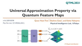
Universal Approximation Property via Quantum Feature Maps ---- The quantum Hilbert space can be used as a quantum-enhanced feature space in machine learning (ML) via the quantum feature map to encode classical data into quantum states. We prove the ability to approximate any continuous function with optimal approximation rate via quantum ML models in typical quantum feature maps. --- Contributed talk at Quantum Techniques in Machine Learning 2021, Tokyo, November 8-12 2021. By Quoc Hoan Tran, Takahiro Goto and Kohei Nakajima

1. Universal Approximation Property via
Quantum Feature Maps
Quoc Hoan Tran*,Takahiro Goto*, and Kohei Nakajima
Physical Intelligence Lab, UTokyo
QTML2021
arXiv:2009.00298
Phys. Rev. Lett. 127, 090506 (2021)
(*) Equal contribution

2. The future of intelligent computations
2/20
Bits
Qubits
Neurons Quantum
mind
Quantum computing
High Efficiency + Fragile
Neural networks
Versatile + Adaptive + Robust
Two rising fields can be complementary
Converge to an adaptive platform:
Quantum Neural Networks

3. QNN via Quantum Feature Map[1,2]
3/20
[1] V. Havlíček et al., Supervised Learning with Quantum-Enhanced Feature Spaces, Nature 567, 209 (2019)
[2] M. Schuld and N. Killoran, Quantum Machine Learning in Feature Hilbert Spaces, Phys. Rev. Lett. 122, 040504 (2019)
[3] Y. Liu et al., A Rigorous and Robust Quantum Speed-Up in Supervised Machine Learning, Nat. Phys. 17, 1013 (2021)
Input Space 𝒳
Quantum
Hilbert space
𝒙
|Ψ 𝒙 ⟩
Access via Measurements
or Compute Kernel
Or at least the same
expressivity as classical
𝜅 𝒙, 𝒙′ = ⟨Ψ(𝒙)|Ψ(𝒙′)⟩
Heuristic
Quantum Circuit Learning
(K. Mitarai, M. Negoro,M. Kitagawa,
and K. Fujii, Phys. Rev.A 98, 032309)
◼ For a special problem, a formal quantum advantage[3] can
be proven (but is neither “near-term” nor practical)
◼ We expect quantum feature maps to be more
expressive than classical counter parts

4. Universal Approximation Property (UAP)
4/20
𝑥1
𝑥2
𝑤1
𝑤2
𝑤𝐾
𝑦
◼ Feed-forward NN with one hidden layer can approximate any
continuous function* on a closed and bounded subset of ℝ𝑑
to
arbitrary 𝜀 (Hornik+1989, Cybenko+1989)
* This belongs to a larger class of any Borel measurable function (beyond this talk)
➢ Given enough hidden units with any
Squashing Activation Functions (Step,
Sigmoid,Tanh, Relu)
➢ Extensive extensions to non-continuous
activation function, resource evaluation

5. UAP of Quantum ML models
5/20
Data Re-uploading
Adrián Pérez-Salinas et al., Data re-uploading for a universal quantum
classifier, Quantum 4, 226 (2020)
Expressive power via a partial
Fourier series
M, Schuld, R. Sweke and J. J. Meyer, Effect of data encoding on the expressive power
of variational quantum-machine-learning models, Phys. Rev.A 103, 032430 (2021)
𝑓𝜽 𝒙 = ෍
𝜔∈Ω
𝑐𝜔 𝜽 𝑒𝑖𝜔𝒙
Our simple but clear questions
◼ UAP in the language of observables
and quantum feature maps
◼ How well the approximation could
perform?
◼ How many parameters it needs (vs.
classical NNs)?

6. QNN via Quantum Feature Map
◼ Choosing W is equivalent to selecting suitable observables
6/20
◼ The output is a linear expansion of the basis functions with a
suitable set of observables
𝜓𝑖 𝒙 = Ψ 𝒙 𝑂𝑖 Ψ 𝒙 𝑓 𝒙; Ψ, 𝑶, 𝒘 = ෍
𝑖=1
𝐾
𝑤𝑖𝜓𝑖 𝒙
[1]V. Havlíček et al., Supervised Learning with Quantum-Enhanced Feature Spaces, Nature 567, 209 (2019)
𝑤𝛽 𝜽 = Tr 𝒲† 𝜽 𝑍⊗𝑁𝒲 𝜽 𝑃𝛽 𝑃𝛽 ∈ 𝐼, 𝑋, 𝑌, 𝑍 ⊗𝑁
𝜓𝛽 𝒙 = Tr Ψ 𝒙 Ψ 𝒙 𝑃𝛽
Pauli-group
Basis functions (expectation)
E.g., Decision function[1] sign
1
2𝑁 ෍
𝛽
𝑤𝛽 𝜽 𝜓𝛽 𝒙 + 𝑏

7. UAP via Quantum Feature Map
𝑓 𝒙; Ψ, 𝑶, 𝒘 = ෍
𝑖=1
𝐾
𝑤𝑖𝜓𝑖 𝒙 ≈ 𝑔 𝒙 ?
Given a compact set 𝒳 ∈ ℝ𝑑
, for any
continuous function 𝑔: 𝒳 → ℝ, can we
find 𝚿, 𝑶, 𝒘 s.t
7/20
UAP. Let 𝒢 be a space of continuous functions 𝑔: 𝒳 → ℝ.The quantum feature framework
ℱ = {𝑓 𝒙; Ψ, 𝑶, 𝒘 } has the UAP w.r.t. 𝒢 and a norm ⋅ if given any 𝑔 ∈ 𝒢; then for any
𝜀, there exists 𝑓 ∈ ℱ s.t. 𝑓 − 𝑔 < 𝜀
Classification capability. For arbitrary disjoint regions 𝒦1, 𝒦2, … , 𝒦𝑛 ⊂ 𝒳, there exists
𝑓 ∈ ℱ s.t. 𝑓 can separate these regions (can be induced from UAP)
𝒳
ℝ
𝒦1
𝒦2
𝑓 ∈ ℱ

8. UAP - Scenarios
Parallel
Sequential
◼ Encode the “nonlinear” property in the basis functions for UAP
1. Using appropriate observables to construct a polynomial
approximation
2. Using appropriate activation functions in pre-processing 8/20

9. Parallel scenario
Approach 1. Produce the “nonlinear” by suitable observables
◼ Basis functions can be polynomials if we choose the
correlated measurement operators
◼ Then we apply the Weierstrass’s polynomial approximation
theorem
𝑈𝑁 𝒙 = 𝑉1 𝒙 ⊗ ⋯ ⊗ 𝑉𝑁 𝒙
𝑉
𝑗 𝒙 = 𝑒−𝑗𝜃𝑗 𝒙 𝑌 𝜃𝑗 𝒙 = arccos( 𝑥𝑘) for 1 ≤ 𝑘 ≤ 𝑑, 𝑗 ≡ 𝑘(mod 𝑑)
𝑂𝒂 = 𝑍𝑎1 ⊗ ⋯ ⊗ 𝑍𝑎𝑁, 𝒂 ∈ 0,1 𝑁
Observables
Basis functions 𝜓𝒂 𝑥 = Ψ𝑁 𝒙 𝑂𝒂 Ψ𝑁 𝒙 = ෑ
𝑖=1
𝑁
2𝑥[𝑖] − 1
𝑎𝑖
Feature map: Ψ𝑁(𝒙) = 𝑈𝑁 𝒙 0 ⊗𝑁
1 ≤ 𝑖 ≤ 𝑑
𝑖 ≡ 𝑖 (𝑚𝑜𝑑 𝑑)
9/20

10. Parallel scenario
Approach 1. Produce the “nonlinear” by suitable observables
Lemma 1. Consider a polynomial 𝑃(𝒙) of the input 𝒙 = 𝑥1, 𝑥2, … , 𝑥𝑑 ∈ 0,1 𝑑 where the
degree of 𝑥𝑗 in 𝑃(𝒙) is less than or equal to
𝑁+(𝑑−𝑗)
𝑑
for 𝑗 = 1, … , 𝑑 𝑁 ≥ 𝑑 ; then there exists a
collection of output weights {𝑤𝒂 ∈ 𝑅|𝒂 ∈ 0,1 𝑁} s.t.
෍
𝒂∈ 0,1 𝑁
𝑤𝒂 𝜓𝒂 𝒙 = 𝑃(𝒙)
Result 1. (UAP in the parallel scenario). For any continuous function 𝑔: 𝒳 → 𝑅
lim
𝑁→∞
min
𝒘
෍
𝒂∈ 0,1 𝑁
𝑤𝒂𝜓𝒂 𝒙 − 𝑔(𝒙)
∞
= 0
※The number of observables ≤ 2 +
𝑁−1
𝑑
𝑑
10/20

11. Parallel scenario
Approach 2. Activation function in pre-processing (straight-forward)
[Huang+, Neurocomputing, 2007] 𝜎: 𝑅 → [−1,1] is nonconstant piecewise continuous function
such that 𝜎(𝒂 ⋅ 𝒙 + 𝒃) is dense in 𝐿2(𝑋).Then, for any continuous function 𝑔: 𝑋 → 𝑅 and any
function sequence 𝜎𝑗 𝒙 = 𝜎 𝒂𝑗 ⋅ 𝒙 + 𝑏𝑗 where 𝒂𝑗, 𝑏𝑗 are randomly generated based on any
continuous sampling distribution,
lim
𝑁→∞
min
𝒘
෍
𝑗
𝑁
𝑤𝑗𝜎𝑗 𝒙 − 𝑔(𝒙)
𝐿2
= 0
We obtain UAP if we can implement the squashing activation function in
pre-processing process (Result 2)
• 𝑈𝑁 𝒙 = 𝑉1 𝒙 ⊗ ⋯ ⊗ 𝑉𝑁 𝒙
• 𝑉
𝑗 𝒙 = 𝑒−𝑗𝜃𝑗 𝒙 𝑌
• 𝜃𝑗 𝒙 = arccos(
1+𝜎(𝒂𝑗⋅𝒙+𝑏𝑗)
2
)
𝜓𝑗 𝑥 = Ψ𝑁 𝒙 𝑍𝑗 Ψ𝑁 𝒙 = ⟨0|𝑒𝑖𝜃𝑗𝑌
𝑍𝑒−𝑖𝜃𝑗𝑌
|0⟩
= 2 cos2(𝜃𝑗) − 1 = 𝜎 𝒂𝑗 ⋅ 𝒙 + 𝑏𝑗 = 𝜎𝑗(𝒙)
11/20

12. Sequential scenario with a single qubit
Finite input set 𝒳 = {𝒙1, 𝒙2, … , 𝒙𝑀}
𝑉 𝒙 = 𝑒−𝜋𝑖𝜃 𝒙 𝑌
→ 𝑉𝑛
𝒙 = 𝑒−𝜋𝑖𝑛𝜃 𝒙 𝑌
Basis functions with the Pauli-Z
𝜓𝑛 𝒙 = 0 𝑉𝑛 †
𝒙 𝑍𝑉𝑛
𝒙 0 = 2 cos2
(𝜋𝑛𝜃(𝒙))
= cos 2𝜋𝑛𝜃 𝒙 = cos(2𝜋{𝑛𝜃 𝒙 })
We can use the ergodic theory
of the dynamical system on M-
dimensional torus
Lemma 3. If real numbers 1, 𝑎1, … , 𝑎𝑀 are linearly independent over ℚ,
then 𝑛𝑎1 , … , 𝑛𝑎𝑀 𝑛∈ℕ is dense in 0, 1 𝑀
.
Result 3. If 1, 𝜃(𝒙1), … , 𝜃(𝒙𝑀) are linearly independent over ℚ, then for
any function 𝑔: 𝒳 → ℝ and for any 𝜀 > 0, there exists 𝑛 ∈ ℕ such that
𝑓
𝑛 𝑥 − 𝑔 𝑥 < 𝜀 for ∀𝑥 ∈ 𝒳
12/20

13. UAP – Approximation Rate
Classical UAP of DNN
inf
𝐰
𝑓
𝒘 − 𝑔 = 𝑂(𝐾−𝛽/𝑑
)
[1] Hrushiksh M Mhaskar. Neural networks for optimal approximation of smooth and analytic functions. Neural Computation, 8(1):164-167, 1996
Optimal rate[3]
[2] Dmitry Yarotsky. Error bounds for approximations with deep Relu networks. Neural Networks, 94:103-114, 2017
[3] Ronald A DeVore. Optimal nonlinear approximation. Manuscripta Mathematica, 63(4):469-478, 1989.
𝐾
𝜀
𝑂(𝐾−𝛼1)
𝑂(𝐾−𝛼2)
𝛼1 < 𝛼2
13/20
The following statement[1,2] holds for continuous activation
function (with 𝐿 = 2), and ReLU (with 𝐿 = 𝑂(𝛽log
𝐾
𝑑
))
➢ 𝑑: input dimension
➢ 𝐾: number of network parameters
➢ 𝛽: derivative order of g
➢ 𝐿: number of layers.
How to describe relative good and bad UAP?
Approximation Rate = Decay rate of appr. error vs.
(better rate)

14. UAP – Approximation Rate
Approximation Rate = Decay rate of appr. error vs.
➢ Number K of observables
➢ Input dimension d
➢ Number N of qubits
𝐾
𝜀
𝑂(𝐾−1/3𝑑)
𝑂(𝐾−1/𝑑)
14/20
In the parallel scenario: 𝐾 = 𝑂 𝑁𝑑
→ 𝜀 = 𝑂 𝐾−1/𝑑
Result 4. If 𝑋 = 0,1 𝑑 and the target function 𝑔: 𝑋 → 𝑅 is Lipschitz continuous w.r.t. the
Euclidean norm, we can construct an explicit form of the approximator to 𝑔 in the parallel
scenario by 𝑁 qubits with the error 𝜀 = 𝑂(𝑑7/6𝑁−1/3). Furthermore, there exist an
approximator with 𝜀 = 𝑂(𝑑3/2𝑁−1)
(optimal rate)

15. Sketch of the proof
Use multivariate Bernstein polynomials for approximating
continuous function g
Number of qubits 𝑁 = 𝑛𝑑 (𝑑: input dimension)
How to create these terms by observables?
15/20

16. Consider the operators for each 𝒑 = (𝑝1, … , 𝑝𝑑)
16/20

17. We choose the following observables
Basis functions
17/20

18. Approximate rate in parallel scenario
We evaluate the approximation rate via the approximation of multivariate
Bernstein polynomials to a continuous function
18/20

19. Approximate rate in parallel scenario
We use the Jackson theorem in higher dimension of the quantitative information on the
degree of polynomial approximation (D. Newman+1964)
Bernstein basis polynomials form a basis of the linear space of 𝑑–variate polynomials
of degree less than or equal to 𝑁 (but we do not know the explicit form)
19/20

20. Summary
◼ UAP via simple quantum feature
maps with observables
◼ Other questions:
◼ Evaluate how well the approximation
could perform (vs. classical scenario)
➢ UAP with other properties of the target function: non
continuous, varied smoothness from place to place
➢ Entanglement and UAP
➢ Approximation rate with the number of layers
(such as in data re-uploading scheme)
Thank you for listening!
20/20
◼ Require a large number of qubits