fracture rougnhess

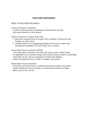
1. FRACTURE MECHANICS
WHAT IS FRACTURE MECHANICS
Fracture mechanics is mechanics
of solids containing planes of displacement discontinuities (cracks)
with special attention to their growth
Fracture mechanics is a failure theory that
1. determines material failure by energy criteria, possibly in conjunction with
strength (or yield) criteria
2. considers failure to be propagating throughout the structure rather than
simultaneous throughout the entire failure zone or surface.
Linear elastic fracture mechanics (LEFM)
is the basic theory of fracture, that deals with sharp cracks in elastic bodies.
It is applicable to any materials as long as the material is elastic except in a vanishingly
small region at the crack tip (assumption of small scale yielding),
brittle or quasibrittle fracture, stable or unstable crack growth
Elastic-plastic fracture mechanics
is the theory of ductile fracture, usually characterized by stable crack growth
(ductile metals) the fracture process is accompanied by formation of large
plastic zone at the crack tip

2. COMPARISON OF THE FRACTURE MECHANICS APPROACH TO THE
DESIGN WITH THE TRADITIONAL STRENGTH OF MATERIALS
APPROACH

3. GOVERNING EQUATIONS OF LINEAR ELASTICITY
In this study we shall consider only statics. Individual particles of the body will be
identified by their coordinates xi (i = 1, 2, 3) in the undeformed configuration.
Displacement field
ui = ui(x1, x2, x3) = ui(xj).
Strain field
ij =
1
2
(ui,j + uj,i) . (1)
Equations of equilibrium
σij,j + Xi = 0 (2)
σij = σji.
Surface tractions
pi = σijnj. (3)
Constitutive equations
σij = Lijkl( kl − 0
ij) (4)
Lijkl = Ljikl = Lijlk.
The fourth-order tensor Lijkl is known as the stiffness tensor. Suppose that a strain
energy density function U( ij) per unit volume volume exists such that
σij =
∂U
∂ ij
. (5)

4. Eqs. (2) and (4) readily provide
Lijkl = Lklij
and that
U =
1
2
Lijkl ij kl. (6)
Providing the strain energy U has a minimum in the stress-free state then Lijkl is
positive definite
Lijkl ij kl > 0 (7)
for all non-zero symmetric tensors ij. It is now possible to invert Eq. (4) to get
ij = Mijklσkl + σ0
ij (8)
Mijkl is known as the compliance tensor. Note that
Mijkl = Mjikl = Mijlk = Mklij
and also
LijrsMrskl =
1
2
(δikδjl + δilδjk) = Iijkl, (9)
where δij is the Kronecker delta and Iijkl represents the fourth-order identity tensor.
Note: we used standard Cartesian tensor notation in which repeated suffixes are summed
over the range 1, 2, 3.

5. AVERAGES
In preparation for evaluation of the overall moduli we first review some basic formulae
for the determination of average stresses and strains. To that end, we assume that the
displacements fields are continuous, and the strain fields are compatible; also, the stress
fields and tractions are continuous and in equilibrium
Consider first an arbitrary homogeneous medium of volume V with the boundary S. In
general, the volume average of a quantity is just the ordinary volume average given by
f =
1
V V
fdV. (10)
Let (x) and σ(x) be certain fields in V . Their volume averages are defined as
=
1
V V
(x) dV σ =
1
V V
σ(x) dV (11)
After applying the divergence theorem we arrive at
ij =
1
2V S
(uinj + ujni)dS (12)
σij =
1
2V S
(pixj + pjxi)dS (13)
Next, consider a heterogeneous elastic medium which consists of a homogeneous matrix
V2 and homogeneous inclusion V1. Evaluation of the above volume averages requires an

6. application of a generalized (but still standard) divergence theorem. Let f be continuous
in V and continuously differentiable in the interior of V1 and V2. We may now apply
the divergence theorem separately to V1 and V2 to conclude that
V
∂f
∂xi
dV +
Σ
[f]mjdS =
S
fnidS (14)
where [f] denotes the jump in the value of f as we travel across Σ from V1 to V2. Now,
assume that perfect bonding exists. When setting f = ui in Eq. (14) we immediately
recover Eq. (12). Since tractions are continuous across Σ
[σij]mj = 0
setting f = σikxj yields Eq. (13). We may now conclude that Eqs. (12) and (13)
apply to any heterogeneous material, generally anisotropic, consisting of a homogeneous
matrix and an arbitrary number of homogeneous inclusions.

7. EXAMPLES 1.1
Consider an arbitrary composite material with outer boundary S
1. Suppose that the composite is loaded by displacements ui on S, which are com-
patible with the uniform strain Eij, i.e. ui = Eijxj (affine displacements). Show
that
< ij >= Eij.
2. Suppose that the composite is loaded by prescribed tractions pi on S, which are
compatible with the uniform stress Σij, i.e. pi = Σijnj. Show that
< σij >= Σij.
3. Let σij be a self-equilibrated stress field (σij,j=0) and ui is a displacement field
associated with strain ij = 1
2
(ui,j +uj,i). Show that if either ui = 0 or σijnj = 0
on the boundary then
V
σij ij dV = 0.
4. For the boundary conditions of Exs. (1) and (2) show that (Hill’s lemma)
< σij ij >=< σij >< ij > and < U >=
1
2
< σij >< ij > .

8. MINIMUM ENERGY PRINCIPLES
We now give a brief review of the classical energy principles as they have been extensively
used in assessing the bounds on the overall elastic properties of composites.
First, consider an arbitrary anisotropic elastic medium Ω with prescribed displacements
ui along its boundary. Let ij, σij, U be the associated strain, stress, and strain energy
density, respectively. The purpose of this investigation is to show that the energy density
U∗
associated with any kinematically admissible displacement field u∗
i is greater than
the energy function U associated with the true solution. Let
∗
ij =
1
2
(u∗
i,j + u∗
j,i) σ∗
ij = Lijkl
∗
ij
U∗
=
1
2
σ∗
ij
∗
ij.
In the next step, calculate the energy of the difference state with displacements (u∗
i −ui),
which is positive
1
2
(σ∗
ij − σij)( ∗
ij − ij) ≥ 0
Therefore,
1
2 Ω
(σ∗
ij
∗
ij − σij ij) dΩ ≥
1
2 Ω
(σ∗
ij ij + σij
∗
ij − 2σij ij) dΩ
Applying Betti’s theorem σ∗
ij ij = σij
∗
ij yields
1
2 Ω
(σ∗
ij
∗
ij − σij ij) dΩ ≥
Ω
σij( ∗
ij − ij) dΩ = 0

9. and finally
Ω
U∗
dΩ ≥
Ω
U dΩ (15)
we recover a special case of the theorem of minimum potential energy.
Next, consider the second boundary value problem with prescribed tractions along the
boundary of the anisotropic solid. Once again, let ui be the required solution and
ij, σij, W be the corresponding strain, stress, and stress (complementary) energy den-
sity function, respectively. Suppose that τij is any statically admissible stress field and
define the associated field ηij
ηij = Mijklτkl.
Again, using the trick of computing the positive energy associated with difference state
1
2
(τij − σij)(ηij − ij) ≥ 0
yields
1
2 Ω
(τijηij − σij ij) dΩ ≥
1
2 Ω
(τij ij + σijηij − 2σij ij) dΩ
Ω
(τij − σij) ij dΩ = 0.
It now follows that
Ω
Mijklτijτkl dΩ ≥
Ω
Mijklσijσkl dΩ, (16)
which is the special case of the theorem of minimum complementary energy.

10. EXAMPLES 1.2
Consider an arbitrary heterogeneous body with outer boundary S.
1. Suppose that the medium is loaded by prescribed displacements ui on S. Then, if
the material is stiffened in any way (keeping the boundary fixed) show that strain
energy increases (Hill’s stiffening theorem).
2. Show that if the stiffness tensor Lijkl is increased by a positive amount, then the
corresponding compliance tensor Mijkl decreases by the positive definite amount.

11. VARIATIONAL PRINCIPLES
Consider an arbitrary anisotropic elastic body Ω loaded by prescribed displacements ui
along a portion of its boundary Γu and and prescribed tractions pi on Γp. The minimum
of total potential energy Π = Ei + Ee is then given by
δΠ = δ(Ei + Ee)
=
Ω
δ ijσij dΩ −
Ω
δuiXi dΩ −
Γp
δuipi dΓ = 0. (17)
Eq. (17) represents the Lagrange variational principle of the minimum of total potential
energy. Principle of the minimum of complementary energy follows from the Castiglian
variational principle and assumes the form
δΠ∗
= δ(E∗
i + E∗
e )
=
Ω
δσij ij dΩ −
Γu
δpiui dΓ = 0. (18)
Note that applying the Lagrange variational principle provides the Cauchy equations
of equilibrium and static (traction) boundary conditions. However, when invoking the
Castiglian variational principle we arrive at the geometrical equations and kinematic
(displacement) boundary conditions.

12. AN ATOMISTIC VIEW OF FRACTURE
It comes out from the assumption that a material fractures when sufficient stress and
work are applied on the atomic level to break the bonds that hold atoms together. The
bond strength is supplied by the attractive forces between atoms.
x0
¢¡¡££¢¤¤¥¥¢¦¦§§¢¨¨
©©¢
¢
¢
¢
¢
¢
!!¢
##¢$$
%%¢
''¢((
))¢00
11¢22
x0
3
3
3
3
3
3
3
3
3
3
3
3
3
34
4
4
4
4
4
4
4
4
4
4
4
4
4
k
Potential
energy
Repulsion
Compression
Attraction
Tension
force
Applied
Bond
energy
force
Cohesive
Bond
energy
Distance
Distance
k
Equilibriun
spacing
λ
σ
σ

13. AN ATOMISTIC VIEW OF FRACTURE - Continue
The bond energy is provided by
Eb =
∞
x0
Pdx (19)
where x0 is the equilibrium spacing and P is the applied force. Assume that the
cohesive strength at the atomic level can be estimated by idealizing the interatomic
force-displacement relationship as one half the period of a sine wave:
P = Pcsin
π(x − x0)
λ
(20)
with the origin defined at x0. For small displacements we get
P = Pc
π(x − x0)
λ
(21)
and the bond stiffness is given by
k =
Pcπ
λ
. (22)
Multiplying both sides of Eq. (22) by the number of bonds per unit area and dividing
by the gage length x0 gives
σc =
Eλ
πx0
σc =
E
π
(23)
where E is the elastic modulus and σc is the cohesive strength.

14. AN ATOMISTIC VIEW OF FRACTURE - Continue
Introduce a surface energy γs resulting from non-equilibrium configuration of atoms on
an arbitrary surface as
2γs =
x0+λ
x0
σ(x)dx ⇒ γs =
1
2
λ
0
σc sin
πx
λ
dx = σc
λ
π
(24)
Note that the surface energy equals one half of the fracture energy since two surfaces are
created when material fractures. Finally, substituting for λ from Eq. (23) into Eq. (24)
and solving for σc gives
σc =
Eγs
x0
. (25)
Example
γs = 1 − 10J/m2
, E = 1011
− 1012
N/m2
, x0 = 2 ∗ 10−10
m ⇒ σc = E/5.
Recall, that the theoretical cohesive strength is approximately E/π. But practical and
experimental observations suggest that the true fracture strength is typically three to
fours orders of magnitude below the theoretical value. This discrepancy, as pointed out
already by Leonardo da Vinci, Griffith, and others, is due to flaws (defects) in these
materials. As shown by the previous derivation, fracture cannot occur unless the stress
at the atomic level exceeds the cohesive strength of material. Thus flaws must lower the
global strength by magnifying the strength locally −→ concept of stress concentration.
Typical flaws include: defects, cracks, secondary phases, etc.

15. STRESS IN AN INFINITE PLATE WITH AS A CIRCULAR HOLE
This problem can be solved by introducing the Airy stress function in polar coordinates.
σ
σ
x
y
F =
xσ
2
2
+ =
σ σ
σσ
I II
2a
An infinite flat plate subjected to remote tensile stress
Airy stress function

16. STRESS IN AN INFINITE PLATE WITH AN ELLIPTICAL HOLE
The first quantitative evidence for the stress concentration factor was provided by Inglis,
who analyzed elliptical holes in flat infinite plates.
¢¡¡
£
£
£
£
£
£
£
£
£
£
£
£
£
£
£
£
£
£
¤
¤
¤
¤
¤
¤
¤
¤
¤
¤
¤
¤
¤
¤
¤
¤
¤
¤
¥
¥
¥
¦
¦
¦
2a
σ
σ
2b ρ
A
Elliptical hole in a flat plate
Inglis (1913) found that the maximum net section stress at point A (see the figure
above) is provided by
σA = σ 1 +
2a
b
(26)
where σ is the nominal (remote) stress. Note that if a = b (circle) then σA = 3σ.
When defining the radius of curvature ρ = b2
/a the maximum local stress σA attains
the form
σA = σ 1 + 2
a
ρ
and if a ρ σA = 2σ
a
ρ
. (27)
The above criterion suffers from the major drawback. In particular, if ρ → 0 then
σA → ∞. This is not realistic, because no material can withstand infinite stress.

17. E.g., in ductile materials (metals), the infinite stress is avoided by yielding and non-
linear deformation −→ blunting of the crack tip. Moreover, accepting an infite stress
imediatelly suggests that localized yielding will occure at the crack tips for any nonzero
value of the remote stress σ. The commonly employed failure criterion such as Von
Mises predicts yielding for any load level and is therefore inadequate for jugging the
crack stability −→ some local criterion based on fracture mechanics is needed.
STRESS IN AN INFINITE PLATE WITH AN ELLIPTICAL HOLE -
Continue
An infinitely sharp crack in a continuum is a mathematical abstraction that is not rele-
vant to real materials, which are made of atoms. In the absence of plastic deformation,
the minimum radius a crack tip can have is on the order of the atomic radius. Thus
setting ρ = x0 yields
σA = σA = 2σ
a
x0
. (28)
Assuming that fracture occurs when σA = σc results in the expression for the remote
stress at failure as
σf =
Eγs
4a
. (29)
Note that Eq. (29) must be viewed as a rough estimate of failure stress, because the
continuum assumption of Inglis analysis breaks at the atomic level.
Example
γs = 1−10J/m2
, E = 1011
−1012
N/m2
, x0 = 2∗10−10
m a = 5000x0 ⇒ σf = E/700.

18. GRIFFITH ENERGY CRITERION
The paradox of a sharp crack motivated Griffith to develop a fracture theory based on
energy rather than local stress. He observed that to introduce a crack into an elastically
stressed body one would have to balance the decrease in potential energy (due to the
release of stored elastic energy and the work done by external loads) and the increase
in surface energy resulting from the presence of the crack which creates new surfaces.
Recall, that surface energy arises from the non-equilibrium configuration of atoms at
any surface of a solid. Likewise he reasoned that an existing crack would grow by some
increment if the necessary surface energy was supplied to the system.
According to the First law of thermodynamics, when a system goes from a non-
equilibrium state to equilibrium, there will be a net decrease in energy. In 1920 Griffith
applied this idea to the formation of crack. To that end, suppose that the crack is
formed by the sudden annihilation of the tractions acting on its surface. At the same
instant, the strain and thus the potential energy posses their original values. But in
general, this new state is not in equilibrium. It is not a state of equilibrium, then, by
the theorem of minimum of potential energy, the potential energy must be reduced by
the attainment of equilibrium. If it is a state of equilibrium the energy does not change.
Therefore, a crack can form (or an existing crack can grow) only if such a process
causes the total energy to decrease or remain constant. Thus the critical condition for
the fracture can be defined as the point at which crack growth occurs under equilibrium
conditions. In mathematical terms the above statement reads
dE
dA
=
dΠ
dA
+
dWs
dA
= 0. (30)

19. GRIFFITH ENERGY CRITERION - Continue
Let’s follow Griffith’s treatment.
B
2a
σ
σ
Griffith crack
Through−thickness crack in an infinite plate
subject to a remote tensile stress
Griffith wrote an expression for the change in total energy that would result from the
introduction of an Inglis crack into an infinitely large, elastically stressed body as a sum
of the decrease in potential energy and the increase in surface energy
E − E0 = −
πσ2
a2
B
E
+ 4aBγs (31)
where the first term on the right hand side represents the decrease in potential energy
and the second term is the increase in surface energy.
σ
σ
σ
σ
I
2a
B
II

20. GRIFFITH ENERGY CRITERION - Continue
Introducing Eq. (31) into Eq. (30) gives
2γs =
πσ2
a
E
(32)
Thus Eq. (32) provides the remote fracture stress at failure in the form
σf =
2Eγs
πa
. (33)
Note that the second derivative of Π
d2
Π
da2
= −
2πσ2
B
E
(34)
is always negative. Therefore, any crack growth will be unstable (as the crack length
changes from the equilibrium length, the energy will always decrease) and the crack will
continue to run.
Note that the Griffith model, Eq. (31), applies only to linear elastic material behavior.
Thus the global behavior of the structure must be linear. Any nonlinear effects such as
plasticity must be confined to a small region near the crack tip.

21. GRIFFITH ENERGY CRITERION - Continue
Note, that the Griffith criterion applies to ideally brittle materials containing sharp
cracks as it assumes that the work required to create new surfaces is proportional to
the surface energy only. Eq. (33), however, can be generalized for any type of energy
dissipation by introducing the fracture energy wf
σf =
2Ewf
πa
. (35)
where wf could include plastic, viscoelastic, viscoplastic and other effects, depending
on material. For the linear elastic solid with the plastic zone confined to a small region
near the crack tip the fracture energy is constant. In many ductile materials, however,
the fracture energy increases with with the crack growth. In such a case, the energy
required for a unit advance of the crack is called the crack growth resistance R.
¢¡¡££¢¤¤
¥¥¢¦¦§§¢¨¨
©©¢¢
¢¢
¢¢
!!¢##¢$$%%¢''¢((
))¢0011¢2233¢4455¢66
77¢8899¢@@
AA¢BBCC¢DD
EE¢FFGG¢HH
II¢PPQQ¢RR
SS¢TTUU¢VV
WW¢XXYY¢``
aa¢bbcc¢dd
ee¢ffgg¢hhii¢ppqq¢rr
ss¢ttuu¢vvww¢xxyy¢€€
¢‚‚ƒƒ¢„„
……¢††‡‡¢ˆˆ
w =f
γs
w =f
γs
‰
‰
‰
‰
‰
‰
‰
‰
‰
‰
‰
‰
‰
‰
‰
‰
‰
‰
‰
‰
‰
‰
‰
‰
‰
‰
‰
‰
‰
‰
‰
‰
‰
‰
‰
‰
‰
‰
‰
‰
‰
‰
‰
‰
‰
‰
‰
‰
‰
‰
‰
‰
‰
‰
‰
‰
‰
‰
‰
‰
‰
‰
‰
‰
‰
‰
‰
‰
‰
‰
‰
‰
‰
‰
‰
‰
‰
‰
‰
‰
‰
‰
‰
‰
‰
‰
‰
‰
‰
‰
‰
‰
‰
‰
‰































































































w =f
γs
+ γp
projected area
true area
Crack broken
bonds Ideally brittle material
crack propagation plastic deformation
quasi−brittle elastic−plastic material
brittle material with crack meandering and branching

22. GRIFFITH ENERGY CRITERION - Continue
Example
a1
ρσ2=σ local
a1
ρσ2=σ local
2a
σ
σ
2a1
microcrackthrough−thickness crack
macroscopic
ρ
sharp penny−shaped
A flat plate made from a brittle material contains a macroscopic through-thickness
crack with half length a1 and notch tip radius ρ. A sharp penny-shaped microcrack
with radius a2 is located near the crack tip of the larger flaw. Estimate the minimum
size of the microcrack to cause failure in the plate when the Griffith equation is satisfied
by the global stress and a1.
¡
¡
¡
¡
¡
¡
¡
¡
¡
¡
¡
¡
¡
¡
¡
¡
¡
¡
¡
¡
¡
¡
¡
¡
¡
¡
¡
¡
¡
¡
¡
¡
¡
¡
¡
¡
¡
¡
¡
¡
¡
¡
¡
¡
¡
¡
¡
¡
¡
¡
¡
¡
¡
¡
¡
¡
¡
¡
¡
¡
¡
¡
¡
¡
¡
¡
¡
¡
¡
¡
¡
¡
¡
¡
¡
¡
¡
¡
¡
¡
¡
¡
¡
¡
¡
¡
¡
¡
¡
¡
¡
¡
¡
¡
¡
¡
¡
¡
¡
¡
¡
¡
¡
¡
¢
¢
¢
¢
¢
¢
¢
¢
¢
¢
£
£
£
£
£
£
£
£
£
£
σ
σ
a
A penny−shaped (circular) crack imbedded
in a solid subjected to remote tensile stress
Note that σf for a penny-shaped crack is given by
σf =
πEγs
2(1 − ν2)a
. (36)

23. ENERGY RELEASE RATE
In 1956 Irwin proposed an energy approach equivalent to Griffith model but more suitable
for solving engineering problems. He introduced an energy release rate G as a measure
of the energy available for an increment of crack extension
G = −
dΠ
dA
or G = −
1
B
dΠ
da
(37)
where B is the thickness of a plane structure. Note that the term rate does not refer
to a derivative with respect to time. G is the rate of change in potential energy with
respect to crack area. G, as it follows from the derivative of a potential, is also called
the crack extension force or the crack driving force.
Consider again the Griffith crack.
B
2a
σ
σ
Griffith crack
Through−thickness crack in an infinite plate
subject to a remote tensile stress
Recall Eq. (31) and write
−
dΠ
dA
= G =
πσ2
a
E
[N/m]. (38)
Thus the crack extension occurs when G reaches a critical value Gf = 2wf , where Gf
is a measure of the fracture toughness. Accepting the hypotheses of elastic fracture
renders Gf constant.

24. ENERGY RELEASE RATE - load control test vs. displacement control test
First consider a crack plate that is dead loaded. Since the load is fixed at P the structure
is said to be load controlled.
1
2
¡
¡
¡
¡
¡
¡
¡
¡
¡
¡
¡
¡
¡
¡
¡
¡
¡
¡
¡
¡
¡
¡
¡
¡
¡
¡
Load P
a
a
a+da
Displacement
∆ ∆d∆+
dU= Pd∆
P
The potential energy of an elastic body is given by
Π = U − A (39)
where U is the strain energy stored in the body and W represents the work done by
external forces. For the present loading conditions we have
U = Ei =
∆
0
Pd∆ =
1
2
P∆ (40)
A = −Ee = P∆ (41)
The energy release rate (fracture energy) is thus provided by
G =
1
B
dU
da P
=
P
2B
d∆
da P
. (42)

25. Since the compliance C of the structure assumes the form
C =
∆
P
and
d∆
da
= P
dC
da
, (43)
we finally arrive at
G =
P2
2B
dC
da
. (44)
Note that under the load controlled conditions the energy required for the crack exten-
sion is supplied by the applied load.
As a next step consider a loading case in which the displacement is fixed. The structure
is displacement controlled.
¡
¡
¡
¡
¡
¡
¡
¡
¡
¡
¡
¡
¡
¡
¡
¡
¡
¡
¡
¡
¡
¡
¡
¡
¡
¡
¢
¢
¢
¢
¢
¢
¢
¢
¢
¢
¢
¢
¢
¢
¢
¢
¢
¢
¢
¢
¢
¢
¢
¢
¢
¢
£
£
£
£
£
£
£
£
£
£
£
£
£
£
£
£
£
£
£
£
£
£
£
£
£
£
Load P
a
a
a+da
∆
∆
−dU −dP
Displacement
When the structure is displacement controlled the external work supplied to the structure
is zero, and therefore A = 0 and Π = U. The energy release rate is then given by
G = −
1
B
dU
da ∆
= −
∆
2B
dP
da ∆
. (45)

26. With the help of Eq. (43) we get
∆ = PC and
dP
da
= −
∆
C2
dC
da
(46)
and finally
G =
P2
2B
dC
da
. (47)
Note that under the displacement controlled conditions the energy required for the crack
extension is supplied by the strain energy.
After comparing Eqs. (44) and (47) we see that the energy release rate, is the same as
defined in Eq. (37), for both load and displacement control and also
dU
da P
= −
dU
da ∆
(48)

27. ENERGY RELEASE RATE - continue
EXAMPLE:
determine the energy release rate for a double cantilever beam (DCB) specimen
¡
¡
¡
¡
¡
¡
¡
¡
¢
¢
¢
¢
¢
¢
¢
¢
£
£
£
£
£
£
£
£
¤
¤
¤
¤
¤
¤¥
¥
¥
¥
¥
¥
¦¦¦§§§
¨
¨
¨
¨
¨
¨
¨
¨
¨
¨
¨
¨
¨
¨©
©
©
©
©
©
©
©
©
©
©
©
©
©
a
a
P
P
P
∆ ∆
2
Solution: Suppose that the crack is sufficiently deep. This assumption allows application
of the beam theory for the derivation of crack opening at the point of the applied load.
Recall
∆
2
=
Pa3
3EI
I =
1
12
Bh3
∆ = CP
C =
2
3
a3
EI
Substituting C into Eq. (47) gives
G =
P2
2B
dC
da
=
12P2
a2
B2h3E
. (49)

28. INSTABILITY AND THE R-CURVE
According to definition crack extension occurs when G = 2wf = R, where R is called
the material resistance to crack extension. Depending on how G and R vary with the
crack size the crack growth may be stable or unstable as shown in the figure below,
which corresponds to a response of the Griffith crack.
stable
unstable
instability
R
R
a0
a0 ac
σ
σ
σ
σ
σ
1
2
3
1
2
G G, ,
G
R
RGfG
Gf
FLAT R−CURVE RISING R−CURVE
crack size crack size
A plot of R versus crack extension is called a resistance or R curve. The corresponding
plot of G versus crack extension is the driving force.
Condition for the stable crack growth
G = R
dG
dR
≤
dR
da
(50)
Condition for the unstable crack growth
dG
dR
dR
da
(51)

29. INSTABILITY AND THE R-CURVE - continue
Some final comments
When the resisting curve is flat, one can define a critical value of energy release rate,
Gf , unambiguously. A material with a rising R curve, however, cannot be uniquely
characterized with a single toughness value. According to Eq. (51) a flaw structure fails
when the driving force curve is tangent with R curve, but this point of tangency depends
on the shape of the driving force, which depends on configuration of the structure.
The R curve for an ideally brittle material is flat because the surface energy is an
invariant property. However, when nonlinear material behavior accompanies fracture,
the R curve can take on a variety of shapes.
Materials with rising R curves can be characterized by the value of G at initiation of
crack growth. This value, however, characterizes only the onset of crack growth and
provides no information on the shape of the R curve.
Ideally, the R curve, should only be a property of the material and not depend on the
size or shape of the crack body. Much of fracture mechanics assumes that the fracture
toughness is material property.

30. ENERGY RELEASE RATE - THE GENERAL ENERGY BALANCE
Consider a body with a preexisting crack loaded up to a certain level at which the crack
advances an elemental length δa in its own plane. The required energy δWF
is given
by
δWF
= RBδa, (52)
where B is the plate thickness and R represents the crack growth resistance. When
R is a material property not dependent on the crack history, flat R curve, notation
R = Gc is often adopted. Hereafter, consider a quasistatic process and suppose that
the only energy-consuming process is fracture. Thus the available energy for fracture,
or (elemental energy release δWR
), reads
δWR
= GBδa = δW − δU, (53)
where δW represents, in the infinitesimal process, the total energy supplied to the struc-
ture (external work), and δU corresponds to the elastic energy stored in the structure.
The specific available energy G (energy release rate) is a measure of energy available for
an increment of crack extension. The energy balance at the onset of fracture requires
Gδa = Rδa. (54)
Note that G is a state function which depends on the instantaneous geometry and
boundary conditions but not how they were attained in the fracture process. G is path
independent.

31. ENERGY RELEASE RATE - continue
Elastic
P+dP
du
a da
Elastic
P
a
u
INITIAL SOLUTION
P − applied load
u − point load displacemet
CO−PLANAR CRACK GROWTH
UPON FURTHER LOADING

32. ENERGY RELEASE RATE FROM THE PRINCIPLE OF VIRTUAL
DISPLACEMENTS
The primary unknowns (independent variables) in the principal of virtual work are equi-
librium displacements which follow from the solution of the elastic problem. The asso-
ciated equilibrium forces, P = P(u, a), can be determined by elastic equilibrium of the
structure.
Consider an elastic body with a crack length a subjected to virtual displacement δu.
First, suppose that there is no crack growth. Hence
δW − δ[U]a = 0. (55)
Next, consider a general process at which both u and a may vary. Then Eq. (53) attains
the form
GBδa = P(u, a)δu −
∂U(u, a)
∂u a
δu +
∂U(u, a)
∂a u
δa . (56)
where P(u, a) is the load and u is the point load displacement. When considering
equilibrium variation at δa = we arrive at the second Castigliano’s theorem
P(u, a) =
∂U(u, a)
∂u a
. (57)
Eq. (56) together with Eq. (57) yield
G = G(u, a) = −
∂U(u, a)
∂a u
. (58)

33. ENERGY RELEASE RATE FROM THE PRINCIPLE OF VIRTUAL FORCES
The primary unknowns (independent variables) in the principal of virtual forces are
equilibrium forces (stresses).
Starting with the complementary energy U∗
given by
U∗
= Pu − U, (59)
denoting u = u(P, a), U∗
(P, a) and considering an equilibrium process in which both
P and a may vary, and using Eq. (53) we get
GBδa = −u(P, a)δP +
∂U∗
(P, a)
∂P a
δP +
∂U∗
(P, a)
∂a u
δa . (60)
When considering equilibrium variation at δa = we arrive at the first Castigliano’s
theorem
u(P, a) =
∂U∗
(P, a)
∂P a
. (61)
Finally, Eqs. (60) and (61) give
G = G(P, a) =
∂U∗
(P, a)
∂a P
. (62)

34. GRAPHICAL REPRESENTATION OF FRACTURE PROCESS
GB∆a = area(OAB ) =
1
2
P(AB ) =
1
2
P [PC(a + ∆a) − PC(a)] =
1
2
P2
C (a)∆a

35. GENERAL NEAR-TIP FIELDS. STRESS INTENSITY FACTORS
For certain cracked configurations subjected to external forces, it is possible to derive
closed-form solutions for the stresses in the body, assuming linear elastic material be-
havior. The early works on this subject are due to Westergaard and Irwin. Irwin, in
particular, proved that so-called local approach, in which the essentials of LEFM are
formulated in terms of stresses close to the crack tip, is essentially equivalent to the
Griffith energetic (or global) approach.
σxx
τxy
τyx
σyy
x
y
θ
crack
When defining a polar coordinate system (r, θ) with the origin at the crack tip the stress
field in any linear elastic cracked body can be written as
σij =
k
√
r
fij(θ) + other terms (63)
where k is a constant and fij is dimesionless function of θ. As evident from Eq. (63)
the stress near the crack tip varies with 1/
√
r, regardless of the configuration of the
cracked body. Note that when r −→ 0 the stress approaches to ∞. In other words,
when a body contains a crack, a strong concentration develops around a crack tip.
However, for linear elastic material this stress concentration has the same distribution
close to the crack tip regardless of the size shape and specific boundary conditions of
the body. Only the intensity of the stress concentration varies. For the same intensity,
the stresses around the crack tip are identical.

36. CENTER CRACKED INFINITE PANEL
σ
8
σ
8
σ
8
σ
8
x
x
1
2
2a
For the center cracked infinite panel loaded by remote normal stress σ∞
in all directions
Griffith showed that the normal stress σyy along the uncracked part of the crack plane
(y = 0, x2
− a2
0) is given by
σyy = σ∞ |x|
√
x2 − a2
. (64)
Introducing the polar coordinate, setting θ = 0, x − a = r, x = r + a, x + a =
r + 2r, x2
− a2
= (x + a)(x − a), and expanding the term (1 + r/a)/ (1 + r/2a) via
Taylor series we get
σyy =
σ∞
√
a
√
2r
1 +
3r
4a
−
5r2
32a2
. . . . (65)
The term in the brackets tends to 1 when r a. Recall Eq. (63) to see that in this
particular case we have
k =
σ∞
√
a
√
2
. (66)

37. STRESS INTENDITY FACTOR - THREE TYPES OF LOADING
There are three types of loading that a crack can experienced.
1. Mode I: principal load is applied to the crack plane, tends to open the crack
2. Mode II: in-plane shear loading, tends to slide one crack face with respect to the
other in its own plane
3. Mode III: out-of-plane shear loading, tends to slide one crack face with respect
to the other out of plane
A crack body can be loaded in any one of these modes, or combination of them.
Nevertheless, each mode produces the 1/
√
r singularity at the crack tip, but the pro-
portionality constant k and function fij in Eq. (63) depend on a specific mode.
It is customary to define k in terms of the stress intensity factor K and write
K = k
√
2π. (67)
Eq. (63) thus receives the form
limr→0σ
(I,II,III)
ij =
K(I,II,III)
√
2πr
f
(I,II,III)
ij (θ) K[Nm−1/2
] (68)
where I, II, III refer to individual loading modes. Note that individual contributions
to a given stress component are additive
σtotal
ij = σ
(I)
ij + σ
(II)
ij + σ
(III)
ij .
However
Ktotal=KI + KII + KIII.

38. STRESS CONCENTRATION FACTOR - THREE TYPES OF LOADING
σyy
π2 r
KIσ
8
θ = 0y
x , r
singularity
dominated zone
crack
When θ = 0, the shear stress is zero and crack plane is a principal plane for pure Mode
I loading. Then the stresses, in the close vicinity of the crack tip, assume the form
σ(I)
xx = σ(I)
yy =
KI
√
2πr
. (69)
Note that Eq. (69) is only valid near the crack tip, where the 1/
√
r singularity dominates
the stress field. Stresses far from the crack tip are governed by the remote boundary
conditions. Therefore, the singularity dominated zone is defined as a region where
Eq. (69), or more general Eq. (68), describes the crack tip stresses. Thus the stresses
near the crack tip increase in proportion to K (K defines the amplitude of the crack
tip singularity).
As intimated in the introductory part, for linear elastic material the stress concentration
has the same distribution close to the crack tip regardless of the size shape and specific
boundary conditions of the body. Thus the stress intensity factor K completely defines
the crack tip conditions (single parameters description of the crack tip conditions).

39. RELATIONSHIP BETWEEN K AND G
1. Energy release rate G: quantifies the net change in potential energy due to
increment of crack extension, global parameter
2. Stress intensity factor K: characterizes the stresses, strains and displacement
fields near the crack tip, local parameter
B
2a
σ
σ
Griffith crack
Through−thickness crack in an infinite plate
subject to a remote tensile stress
In the limit of LEFM parameters G and K are uniquely related. As an example, consider
again a through crack in an infinite plate subject to a uniform stress. In this particular
case we have
G =
πaσ2
E
KI = σ
√
πa
and therefore
G =
K2
I
E
, (70)
where E = E for plane stress and E = E
1−ν2 for plane strain.

40. RELATIONSHIP BETWEEN K AND G - CRACK CLOSURE ANALYSIS
a∆
uy
y
x
crack
Closure
stress
To arrive at a general relationship between G and K we follow Irwin and assume that
the energy release rate G associated with the advancement of crack ∆a can be linked
to the work required to close the crack in this region. According to definition
G = lim∆a→0
∆U
∆a P
(71)
where ∆U is the work of crack closure.

41. CRACK TIP PLASTICITY
Recall that the LEFM applies to sharp cracks. The assumption of sharp cracks, however,
leads to the prediction of infinite stresses at the crack tip. On the other hand, stresses
in real materials are finite because the crack tip radius is finite (recall an atomic view
on fracture). In addition, inelastic deformation, e.g., plasticity in metals, crazing in
polymers or damage in concrete, results in further reduction of crack tip stresses −→
modification of the LEFM to account for the crack tip yielding.
σyy
π2 r
KIσ
8
θ = 0y
x , r
singularity
dominated zone
crack
plastic zone
If the plastic zone at the crack tip is sufficiently small (confined within the singularity
dominated zone), there are two simple approaches available that provide corrections to
the LEFM:
1. the Irwin approach
2. the strip yield model
Note: although the term plastic zone usually applies to metals it will be used here to
represent the inelastic crack tip behavior in more general sense.

42. THE IRWIN APPROACH
ry
θ = 0
crack
r
σyy
σYS
rp
Elastic
Elastic−plastic
1. First-order estimate of the plastic zone size: consider the crack plane (θ = 0) and
suppose that the boundary between elastic plastic behavior occurs when the stress
σyy given by Eq. (69) satisfies the yield criterion (σyy = σY S for plane stress).
Thus substituting the yield stress σyy into Eq. (69) and solving for r gives a first
order estimate of plastic zone size in the form
ry =
1
2π
KI
σY S
2
(72)
Flaw: the analysis is based on purely elastic crack tip analysis
2. Second-order estimate of the plastic zone size: note that when yielding occurs
the stresses must redistribute ahead of the crack tip to satisfy equilibrium. To
that end, consider a simple force balance to get
σY Srp =
ry
0
σyydr =
ry
0
KI
√
2πr
dr =
KI
√
2πr


r
1
2
1
2


ry
0
(73)

43. Substituting for ry from Eq. (72) into Eq. (73) gives a second order estimate of
the plastic zone as
rp =
1
π
KI
σY S
2
(74)
which is twice as large as ry, the first order estimate. Note that the redistributed
stress in the elastic region is higher than predicted by Eq. (69), which implies a
higher effective stress intensity factor (Keff ). Irwin found that a good approxi-
mation of Keff can be obtained by placing the tip of the effective crack in the
center of the plastic zone.
ry
σyy
θ = 0
σyy =
. Keff
crack
r
σYS
rp
yπ2 (r − r )
Determination of the effective crack size aeff
1. set aeff = a + ry
2. write Keff = C(aeff )σ
√
πaeff where C(aeff ) is the geometry correction factor
3. iterate within the first two steps to solve for Keff

44. THE STRIP YIELD MODEL - suitable for polymers
The strip yield model was first proposed by Dugdale and Barenblatt. They assumed
a long slender plastic zone at the crack tip in nonhardening material in plane stress.
In further discussion we limit our attention to a through crack in infinite plate. This
model is a classical application of the principle of superposition as it approximates the
elastic-plastic behavior by superimposing two elastic solutions: a through crack under
remote tension and a through crack with closure stresses at the tip.
σYS
2a + 2ρ
2a ρ
2a
x P
The idea is as follows. Since the stresses at the strip yield zone are finite, there cannot
be a singularity at the crack tip (the stress intensity factor at the tip of plastic zone
must be equal to zero). Thus the plastic zone length ρ is found from the condition
that the stress intensity factors from the remote tension and closure stress cancel one
another.
To proceed, consider first a through crack in an infinite plate loaded by a normal force
P applied at a distance x from the center line of the crack. The stress intensities for

45. the two crack tips are then give by
KI(+a) =
P
√
πa
a + x
a − x
KI(−a) =
P
√
πa
a − x
a + x
(75)
In the next step, we identify the force P at a point with the closure stress σY S through
the
P = −σY Sdx
and replace a with a + ρ to arrive at the stress intensity factor from closure stress
Kclosure = −
σY S
π(a + ρ)
a+ρ
a
a + ρ + x
a + ρ − x
+
a + ρ − x
a + ρ + x
dx (76)
Solving this integral yields
Kclosure = −2σY S
a + ρ
π
cos−1 a
a + ρ
(77)
The stress intensity from the remote tensile stress is given by
Kσ = σ π(a + ρ) (78)
Finally, equating Eqs. (77) and (78) gives
a
a + ρ
= cos
πσ
2σY S
(79)

46. Expanding the right hand side of Eq. (79) via Taylor series provides
a
a + ρ
= 1 −
1
2!
πσ
2σY S
2
+
1
4!
πσ
2σY S
4
−
1
6!
πσ
2σY S
6
+ . . . (80)
Neglecting all but the first two terms and solving for the plastic zone size gives
ρ =
π2
σ2
a
2σY S
=
π
8
KI
σY S
2
(81)
Recall the Irwin approach which gives the size of plastic zone rp as
rp =
1
π
KI
σY S
2
and notice that 1/π = 0.318 and π/8 = 0.392. Therefore, the Irwin approach and the
strip yield model predict similar plastic zone sizes. The Keff follows from the strip yield
model after replacing a by a + ρ. This yields for the through crack in the infinite plate
under remote stress
Keff = σ πa sec
πσ
2σY S
(82)
The actual aeff is somewhat less than a + ρ. More realistic estimate of Keff was
derived by Burdekin and Stone
Keff = σY S
√
πa
8
π2
ln sec
πσ
2σY S
2
(83)

47. PLANE STRESS VS. PLANE STRAIN
PLANE STRESS PLANE STRAIN

48. K AS A FRACTURE CRITERION - LOCAL FRACTURE CRITERION FOR
MODE I (KIc)
Here we limit our attention to a pure mode I failure. In the limit of the LEFM the stress
state of the material in the singularity dominated zone (excluding a very small plastic
zone at the crack tip) is uniquely determined by KI. when assuming the material fails
at some combination of local stresses and strains, then the crack extension must occur
at a critical KIc value called fracture toughness. This value is a material constant
independent of the size and geometry of the crack body and may be determined by
performing a fracture test. If certain conditions are met the KI value that provokes
failure is set to KIc. Since the energy release rate is uniquely related to stress intensity,
G also provides a single-parameter description of the crack tip conditions, and Gc, or
Gf is an alternative measure of fracture.
1. Effect of loading mode: the critical stress intensity factor for a given mode is a
material constant, but Kc varies with the loading mode
KIc = KIIc = KIIIc
Under combination of loading modes, an initially straight crack kinks upon frac-
ture and the fracture criteria must give not only the loading combination that
produces the fracture, but also the kink direction. Mixed-mode fracture is still
a subject of an ongoing research. Nevertheless, the vast majority of practical
applications consider only the Mode I fracture.

49. 2. Effect of specimen dimensions: the critical stress intensity factor is a material
constant only when certain conditions are met. Recall, e.g., that a lower degree
of stress triaxiality usually results in higher toughness. Also, the through thickness
constraint may affect the shape of the R curve. In particular, the R curve for a
material in plane strain may be relatively flat (single valued toughness), while the
plane stress R curve usually rises with crack growth.
KI
Thickness
Plane
stress
Plane
strain
Plastic
zoneCritical
Ic
K
3. Limits to the validity of LEFM: according to the American Society for Testing
and Materials (ASTM) standard for KIc the following specimen size requirements
must be met to obtain a valid KIc results in metals:
a, B, (W − a) ≥ 2.5
KI
σY S
2
where a, B, W are the crack size, thickness, and width of the specimen, respec-
tively. The thickness requirement ensures nearly plane strain conditions and the
requirement on in-plane dimensions ensures that the nominal behavior is predom-
inantly linear elastic.

50. SIZE EFFECT - QUANTIFICATION OF FRACTURE MECHANICS SF
In the classical theories based on plasticity or limit analysis (or other theories in which the
material failure criterion is expressed in terms of critical stresses or strains), the strength
of geometrically similar structures is independent of the structure size. However, the
failure behavior of structures made of brittle or quasibrittle material (e.g., concrete) is
usually size dependent. Such failures are said to exhibit size effect. The size effect on
the structural strength is represented by the deviation of the actual load capacity of a
structure from the load capacity predicted by any theory based on critical stresses or
strains.
Fracture mechanics size effect, resulting from the release of stored energy of the struc-
ture into fracture front, is the most important source of size effect. The size effect is,
for design engineers, the most compelling reason for adopting fracture mechanics (Z.P.
Baˇzant).
Since the size effect is understood as the dependence of the structure strength on the
structure size, it is rigorously defined through a comparison of structure strength of
geometrically similar structures of different sizes. The structure strength is commonly
defined as the nominal stress σNu (load divided by a typical cross-sectional area) at the
peak load
σN = cN
P
bD
for 2D similarity σN = cN
P
D2
for 3D similarity (84)
where P is the applied load, b is the thickness in 2D structure, D is the characteristic
dimension of the structure or specimen and cN is a certain coefficient, which may be
set to 1.

51. EXPLANATION OF FRACTURE MECHANICS SIZE EFFECT (Baˇzant)
First, consider a uniformly stressed panel and suppose that fracture propagates via the
formation of a crack band of thickness hf . The load required to propagate the band
follows from energy balance equation, i.e., energy available is equal to the fracture
energy (the energy required for band extension). To that end, assume that due to
presence of crack band the strain energy in the band and cross-hatched area drops
from σ2
N /2E to zero (this region is called the stress relief zone). Next, consider a
geometrically similar panel.

52. It is usually the case, that the larger the panel, the large the crack band and consequently
the larger the cross-hatched area =⇒ in a larger structure, more energy is released in
a strip by the same extension of the crack band. It is usually assumed that the edges
of the specimen are fixed during the crack advance (displacement control), and so the
external work is zero. The condition balancing the total energy released from the stress
relief zone and the fracture energy needed to advance the crack by ∆a reads
b(hf ∆a + 2ka0∆a)
σ2
N
2E
= Gf b∆a (85)
Following Baˇzant we further denote
Bf =
Gf E
hf
= const and D0 =
hf D
2ka0
= const
where f is the tensile strength and D/a0 = const due to geometrical similarity. Com-
bining the above expressions together with Eq. (85) gives the Baˇzant size effect equation
in the form
σNu =
Bf
1 + D/D0
(86)
Note that both Bf and D0 depend on the fracture properties of the material and on
the geometry of the structure, but not on the structure size. Also not that Eq. (86) is
approximate, valid only within a range of about 1:20 for most structures.

53. SIZE EFFECT IN PLASTICITY
Remember that the size effect is defined by comparing geometrically similar structures
of different sizes. The goal here is to investigate the effect of the size on the nominal
strength σNu written as
σNu = cN
Pu
bD
(87)
Consider a reference structure of size D and geometrically similar one of size D = λD,
where λ is the scaling factor and write stresses at an arbitrary point of coordinates
(x1, x2) in terms of nominal stress σN as σij(σN , x1, x2). Next define a set homologous
points of coordinates (x1 = λx1, x2 = λx2). The similitude (podobnost) laws state
that
σij(σN , x1, x2) = σij(σN , x1, x2) with x1 = λx1, x2 = λx2 (88)
ij(σN , x1, x2) = ij(σN , x1, x2) with x1 = λx1, x2 = λx2 (89)
u (σN , x1, x2) = λu(σN , x1, x2) with x1 = λx1, x2 = λx2 (90)
Eqs. (88), (89) and )(90) thus imply that the stress and strain maxima also occur at
homologous points. Therefore, if failure is assumed to occur when the stress or strain
or in case of plasticity a certain function Ψ(σ, ) reaches a critical value, Ψ(σ, ) = Ψc,
then the two similar structures will fail at the same nominal stress (σNu
= σNu ). In
such a case we say that there is no size effect.

54. SIZE EFFECT IN LEFM
Let D be a characteristic length (arm depth in DCB specimen) and all the remaining
dimensions being proportional (length-to-depth ratio for the DCB). To proceed it is
desirable to express G and KI in terms of the variables P or σN , D and α = a/D. In
particular, we write
KI =
P
b
√
D
ˆk(α) = σN
√
Dk(α) and G =
P2
b2DE
ˆg(α) =
σ2
N
E
Dg(α) (91)
where ˆk(α), k(α), ˆg(α), g(α) are dimensionless constants, ˆg(α) = ˆk2
(α), g(α) = k2
(α),
k(α) = ˆk(α)/cN , g(α) = ˆg(α)/c2
N , and α is the relative crack depth.
Consider now a family of geometrically similar plane cracked structures loaded in mode I.
Let a0 and α0 = a0/D are the initial crack and initial relative crack length, respectively.
Suppose that k(α) increases with α (positive geometries), then σN decreases with the
crack advance and the peak load coincides with the onset of crack growth (KI = KIc)
and
σNi
= σNu =
KIc
√
Dk(α0)
σN =
KIc
√
Dk(α)
(92)
to keep KI = KIc during the crack growth. Evidently, since α0 is constant for geomet-
ricaly similar structures, the nominal strength is always proportional to the square root
of the size.

55. Therefore, for similar precracked structures, the nominal strengths are related
D = λD1
σNu
√
D = σNu1 D1
σNu λD1 = σNu1 D1
σNu = λ
−1
2 σNu1 (93)
It follows, from above, that geometrically similar structures following LEFM exhibit the
inverse square root size effect.

56. NONLINEAR FRACTURE MECHANICS (ELASTIC-PLASTIC FM)
Recall that LEFM is only valid as long as nonlinear material behavior is confined to a
small region surrounding the crack tip. There are many materials, however, for which
the applicability of LEFM is impossible or at least suspicious. Therefore, an alternative
fracture mechanics model is required.
Elastic-plastic fracture mechanics applies to materials that exhibit time-independent,
nonlinear behavior (plastic deformation). There are two parameters characterizing the
nonlinear behavior at the crack tip:
1. CTOD - crack tip opening displacement
2. J counter integral
Critical values of CTOD and J give nearly size-independent measures of fracture tough-
ness, even for relatively large amount of crack tip plasticity. Note that there are still
limits to the applicability of J and CTOD, but these limit are much less restrictive than
the validity requirements of LEFM.

57. CTOD - CRACK TIP OPENING DISPLACEMENT
Wells observed that
• There is an important class of structural steels that are too tough to be charac-
terized by LEFM
• Blunting of initially sharp cracks prior to fracture. The degree of crack blunting
increases in proportion to the toughness of the material −→ he proposed the
crack tip opening displacement as a measure of fracture toughness.
Relationship between G and KI and CTOD in the limit of LEFM (small scale yielding)
The Irwin approach
uy =
κ + 1
2µ
KI
ry
2π
ry =
1
2π
KI
σY S
2
δ = 2uy =
4K2
I
πσY SE
=
4G
πσY S
The strip yield model
δ =
1 − ν2
E
K2
I
σY S
plain strain =
G
σY S
δ =
1
E
K2
I
σY S
plain stress =
G
σY S

58. Definition of CTOD
There are a number of alternative definitions of CTOD. The two most common are:
1. the displacement at the original crack tip
2. so called 900
degree intercept
The above two definitions are equivalent if the crack blunts in semicircle.
Laboratory measurements of CTOD
Most laboratory measurements of CTOD have been made on edge-cracked specimens
loaded in three-point bending. When inferring the CTOD from this experiment it is
assumed that the specimen halfs are rigid and rotate about a hinge point. Then,
measuring the crack mouth opening (V ), as is usually the case, enables to compute the
CTOD from a similarity of triangles as
δ
r(W − a)
=
V
r(W − a) + a)
=⇒ δ =
r(W − a)V
r(W − a) + a
(94)
where r is a rotational factor (dimesionless constant between 0 and 1). Note that the
hinge model becomes inaccurate when displacements are primarily elastic. Therefore,
the total displacement is usually separated into elastic and plastic components and the
hinge model is applied only to plastic displacements to get
δ = δel + δpl =
K2
I
mσY SE
+
rp(W − a)Vp
rp(W − a) + a
(95)

59. The plastic rotational factor rp is approximately 0.44 for typical materials (metals) and
test specimens. Note that Eq.(95) reduces to small scale yielding for linear elastic
condition and the hinge model dominates when V = Vp.
Stability criterion for crack growth
The crack is stable as long as
CTOD ≤ CTODc
The determination of CTODc, however, is ambiguous. Usually, the value of CTODin at
the onset of crack growth is measured. In the limit of LEFM this value can be used to
infer the critical value of stress intensity factor KIc (structural steel with low fracture
toughness).
Specimen size requirements
B ≥ 25CTODin
KIc from CTOD
if CTODin =
4
π
K2
Ic
σY SE
then B ≥ 25
4
π
K2
Ic
σY SE
Recall that for LEFM we require
B ≥ 2.5
KIc
σY S
2
It is therefore evident that when inferring KIc from CTOD we may use specimens of
substantially smaller sizes.

60. J CONTOUR INTEGRAL
Rice presented a path-independent contour integral of analysis of cracks and showed
that the value of this integral, called J, is equal to the energy release rate in a nonlinear
elastic body that contains crack. Hutchinson and also Rice and Rosengren further
showed that J uniquely characterizes crack tip stresses and strains in nonlinear material.
Thus the J integral can be viewed as both an energy parameter and a stress intensity
parameter.
J as nonlinear energy release rate
Recall Eq. (37) and write the nonlinear energy release rate in the form
J = −
dΠ
dA
or J = −
1
B
dΠ
da
(96)
Next, consider a cracked plate which exhibits a nonlinear load-displacement curve.
• Load control
Π = U − W = U − P∆ = −U∗
(97)
where U∗
is the complimentary strain energy given by
U∗
=
P
0
∆ dP
Thus substituting Eq. (97) into Eq. (96) provides
J =
dU∗
da P
=
d
da
P
0
∆ dP
P
=
P
0
d∆
da P
dP (98)

61. • Displacement control
Π = U (99)
where the strain energy U is given by
U =
∆
0
P d∆
After introducing Eq. (99) into Eq. (96) we get
J = −
dU
da ∆
= −
d
da
∆
0
P d∆
∆
= −
∆
0
dP
da ∆
d∆ (100)
After inspecting Eqs. (98) and (100) we arrive at
P
0
d∆
da P
dP = −
∆
0
dP
da ∆
d∆ (101)
Recall that in the limit of LEFM
J = G =
K2
E
(102)

62. J as a path-independent line integral
Consider an arbitrary counter-clockwise path (Γ) around the tip of a crack. The J
integral is given by
J =
Γ
w dy − pi
∂ui
∂x
ds (103)
where w is the strain energy density defined as
w =
ij
0
σij d ij (104)
and pi = σijnj are the surface tractions. Rice showed that the value of J is independent
of the path of integration around the crack. Thus J is called a path-independent
integral.
J as a stress intensity factor
Under the assumption of nonlinear elasticity Hutchinson and Rice Rosengren inde-
pendently showed that J characterizes crack tip conditions. They assumed a power
law relationship between plastic strain and stress which in case of uniaxial deformation
reads (Ramberg-Osgood law)
0
=
σ
σ0
+ α
σ
σ0
n
(105)
where σ0 is a reference stress value usually equal to yield stress, 0 = σ0/E, α is a
dimensionless constant, and n is the strain hardening exponent. H R R showed that

63. for J to remain path independent the quantity stress×strain must vary with 1/r near
the crack tip. When limiting our attention to the plastic zone (elastic deformations are
small small compare to elastic ones) Eq. (105) reduces to a simple power law. Stresses
and strains ahead of the crack tip then receive the following forms
σij = k1
J
r
1
n+1
(106)
ij = k2
J
r
n
n+1
(107)
where k1, k2 are proportionality constants. Note that for linear elastic material n = 1
and indeed above equations predict a 1/
√
r singularity as expected.
It can be concluded that J integral defines the amplitude of the HRR singularity, just as
the stress intensity factor characterizes the amplitude of the linear elastic singularity. J
completely describes the conditions within the plastic zone. Thus a structure in small-
scale yielding has two singularity dominated zones: one in the elastic region, where
stress varies as 1/
√
r and one in the plastic zone where stress varies as r−1/(n+1)
.

64. DETERMINATION OF J FOR A STATIONARY CRACK
1. In elastic material J = G and G is uniquely related to the stress intensity factor
2. Application of the line integral definition of J, Eq. (103) - not suitable for exper-
imental measurements
3. Invoking the energy release rate definition of J, Eq. (96) - more suitable for
experimental measurements
Laboratory measurements of J based on energy release rate definition
1. Determination of J by measuring on a series of specimens (Landes and Begly)
2. Determination of J by measuring on a single specimen - unloading compliance
method for monitoring crack growth
A good insight to how determine J experimentally can be provided by an analysis of
an edge cracked plate in bending assuming the plastic region spreads over the total
ligament length. To that end consider a single edge notched bend (SENB) specimen.
Procedure: First split the angle ψ into elastic and inelastic parts as ψ = ψel + ψp If
ψel ψp then
M = σ0B(W − a)2
g(ψp,
σ0
E
, n)
ψp =
v
L
P =
B
L
(W − a)2
σ0h(
v
L
,
σ0
E
, n)

65. When taking the derivative of F with respect to a we get
∂P
∂a
= −
∂P
∂(W − a)
= 2
B
L
(W − a)σ0h(
v
L
,
σ0
E
, n) = −
2P
W − a
(108)
The energy release rate based definition of J gives
J = −
1
B
∂U
∂a ∆=const
= −
1
B
∆
0
∂P
∂a ∆=const
d∆ (109)
Introducing Eq. (108) into Eq. (109) gives
J =
2
B(W − a)
∆
0
Pd∆ =
2Up
B(W − a)
(110)
where factor 2 represents the ratio between J and plastic work Up per a unit area of
the ligament length assuming a unit thickness of the specimen. Let us denoting this
factor in general by η. Then
β =
JB(W − a)
Up
.
From practice we have: η = 2 for SENB specimen and η = 2 + 0.522(1 − a/W) for
CT specimens. When including elastic effects Eq. (110) receives the form
J =
ηelUel
B(W − a)
+
ηpUp
B(W − a)
=
K2
I
E
+
ηpUp
B(W − a)
. (111)

66. CRACK GROWTH RESISTANCE CURVES
Note that many materials with high toughness do not fail catastrophically at a particular
value of J or CTOD. Rather the material displays a rising R curve, where J and CTOD
increase with crack growth. Therefore, the initial crack growth is usually stable preceded
by a small amount of apparent crack growth due to crack blunting. The onset of stable
crack growth can be characterized by JIC (initiation toughness). However, the precise
point at which the crack begins to grow is not well defined so that the definition of
JIC is somewhat arbitrary. More complete description about the fracture behavior of
ductile materials is provided by the entire R-curve.
The relative stability of the crack growth is indicated by the slope of the R curve at a
given amount of crack extension.
Tearing modulus - slope on J resistance (R) curve
TR =
E
σ2
0
dJR
da
(112)
Applied tearing modulus - slope on the driving force
Tapp =
E
σ2
0
dJ
da ∆T
(113)

67. Conditions for crack growth
1. Stable crack growth
J = JR (114)
Tapp ≤ TR (115)
2. Unstable crack growth
Tapp TR (116)
Recall that the point of instability in a material with rising R curve depends on the
size and geometry of the cracked structure. A critical value of J at instability is not a
material property if J increases with crack growth. However, it is usually assumed that
the R curve, including the JIC value, is a material property independent of configuration.
This is a reasonable assumption within certain limitations.

68. DETERMINATION J FOR A GROWING CRACK
We require for the R curve to be a material property independent of configuration.
However, there is a geometry dependence of the R curve influenced by the way in
which J is calculated. There are various ways to compute J that include:
• deformation J → JD - based on the pseudo energy release rate definition of J
• far-field J → Jf - based on the contour integral definition of J
• modified J → modified JD(JM )
Deformation J
Recall that the J integral is based on deformation plasticity (or nonlinear elasticity)
assumption for the material behavior and is only valid for stationary cracks. Consider
now a growing crack which has grown form its initial length a0 to a length a1 and a
corresponding load-displacement curve. The deformation J, however, is related to the
area under the load-displacement curve for a stationary crack, rather than the area under
the actual load-displacement, where the crack length varies. To that end, consider a
deformation path for a stationary crack fixed at a1 (nonlinear elasticity assumed). The
area under this curve is the strain energy in an elastic material which depends only on
the current load and crack length and is not history dependent which is not true for the
actual elastic-plastic material. This energy is given by
UD = UD(P, a) =
∆
0
Pd∆
a=a1
. (117)

69. Thus the J integral for a nonlinear elastic material with a growing crack is given by
JD = −
1
B
∂UD
∂a ∆
=
ηUD
B(W − a)
(118)
or
JD =
K2
I
E
+
ηUD(p)
B(W − a)
(119)
The calculation of UD(p) is usually performed incrementally, since the load-displacement
curve based on deformation theory depends on the crack length.

70. J CONTROLLED FRACTURE
As in the LEFM there are situations when J and thus also CTOD completely character-
izes crack tip conditions. However, there are limits to the validity of fracture mechanics
analyses based on J and CTOD. In particular, such analyses become suspicious when
there is excessive plasticity at the crack tip or significant crack growth. Fracture tough-
ness given in terms of J then depends on the size and geometry of the structure or test
specimen.
Required conditions for J-controlled fracture
• Stationary cracks:
small scale yielding - both K and J uniquely characterize crack tip conditions.
In particular, in the close vicinity to the crack tip there exists the K-dominated
zone where stresses are proportional to 1/
√
r. In the plastic zone the elastic
singularity no longer applies. However, when assuming monotonic, quasistatic
loading there exists a J-dominate zone in the plastic region where the HRR
solution is approximately valid and the stresses vary as r1/n+1
. Finally, the finite
strain occurs within approximately 2δ from the crack tip, where large deformation
invalidates the HRR theory.
elastic-plastic conditions - J is still approximately valid but there is no K field
large scale yielding - the size of the finite strain region becomes significant and
there is no longer region uniquely characterized by J that exhibit a size and
geometry dependence. Single parameter fracture mechanics is invalid.

71. • J-controlled crack growth:
Recall that in elastic material the prior crack growth has no adverse effects since
the local crack tip fields depend only on current conditions. However, in elastic-
plastic material the prior loading history does influence stresses and strains in the
plastic region.
Consider a crack growth under J-controlled conditions. When crack advances
there exists a region behind the growing crack tip where the material unloads
elastically. Also recall that the material in the unloading region violates the
assumptions of deformation plasticity. Just ahead of the crack tip there is a
region of finite plastic strains where single parameter fracture is also invalid since
the loading is highly nonproportional. Therefore, for the crack growth to be J-
controlled both regions must be embedded within a zone of J − dominance.
Otherwise, the measured R-curve is no longer uniquely characterized by J.
In small scale yielding there is always a zone of J dominance as the crack tip
conditions are defined by the elastic stress intensity, which depends only on current
values of load and crack size. There are three distinct stages of crack growth
resistance in small scale yielding:
1. Stage 1 - initial stage associated with crack blunting is essentially stationary
2. Stage 2 - crack begins to grow, stresses and strains are history dependent
and thus influenced by original blunt crack tip during the early stages of
crack growth

72. 3. Stage 3 - steady state conditions are reached when the crack growth well
beyond the initial blunted tip. During steady-state crack growth a plastic
zone of constant size sweeps through the material leaving a plastic wake.
The R-curve is flat - J does not increase with crack extension. If a rising
or falling R curve appears then the local material properties vary with crack
extension. The steady-state limit is usually not observed in laboratory tests
on ductile material - typically the ligament is fully plastic during the crack
growth that violates small scale yielding assumptions. Enormous specimens
would be required to observe steady state growth in tough materials

73. FRACTURE TOUGHNESS TESTING OF METALS