SlideShare uma empresa Scribd logo
1 de 23
Baixar para ler offline
Directed Optimization on Pareto Frontier

                                               Vladimir Sevastyanov1
                                         eArtius, Inc., Irvine, CA 92614, US

                                              EXTENDED ABSTRACT


           New multi-objective optimization technology is presented which considers Pareto frontier as
           a search space for finding Pareto optimal solutions that meet the user’s preferences.
           Typically, 80-90% of points evaluated by new optimization algorithms are Pareto optimal,
           and the majority of them are located in the user’s area of interest on the Pareto frontier. In
           contrast, conventional optimization techniques search for Pareto optimal solutions in the
           entire domain, which increases computational effort by orders of magnitude. New
           optimization technology is represented by two new algorithms: Multi-Gradient Pathfinder
           (MGP), and Hybrid Multi-Gradient Pathfinder (HMGP) (patent pending). MGP is a pure
           gradient-based algorithm; it starts from a Pareto-optimal point, and steps along the Pareto
           surface in the direction that allows improving a subset of objective functions with higher
           priority. HMGP is a hybrid of a gradient-based technique and genetic algorithms (GA); it
           works similarly to MGP, but in addition, searches for dominating Pareto frontiers. HMGP is
           designed to find the global Pareto frontier and the best Pareto optimal points on this frontier
           with respect to preferable objectives. Both algorithms are designed for optimizing very
           expensive models, and are able to optimize models ranging from a few to thousands of design
           variables.


                                                   1. Introduction

L ow computational efficiency and low scalability of current multi-objective optimization algorithms are the biggest
  obstacles in the design optimization practice, which cause engineers to artificially reduce the number of design
variables, and to rely on brute-force methods such as parallelization of optimization algorithms.
     In our opinion, the main reasons for low computational efficiency and low scalability are: (a) searching for
optimal solutions in an entire design space while the search space can be reduced; (b) attempts to maximize the
diversity of optimization results, and to cover the entire Pareto frontier while the user needs a small part of it; (c)
absence of efficient algorithms for estimating gradients.
     In this paper we discuss in detail the limiting issues in current design optimization technologies, and offer a
breakthrough optimization technology which improves algorithms efficiency by orders of magnitude, and provides
equal optimization efficiency for a large variety of task dimensions ranging from a few to thousands of design
variables.

      A. Searching the Entire Design Space
     Multi-objective optimization algorithms can be classified in the following way: algorithms based on uniformly
distributed sequences such as Monte Carlo algorithm, genetic algorithms, and gradient based algorithms. The
algorithms have different levels of convergence and computational efficiency, which can be characterized, for
instance, by the ratio between the total number of model evaluations and the number of Pareto optimal points found.
However, most of the algorithms of multi-objective optimization perform a search for Pareto optimal points in the
entire design space.


1
    Chief Executive Officer

                                                              1
                                      American Institute of Aeronautics and Astronautics
Let’s consider the benchmark (1) with two objective functions and two design variables.

                                 Minimize       f1 = x1
                                 Minimize       f 2 = 1 + x2 − x1 − 0.1 ⋅ sin( 3π ⋅ x1 )
                                                           2
                                                                                                         (1)
                                 0 ≤ x1 ≤ 1; − 2 ≤ x2 ≤ 2

    The following FIG.1 and FIG.2 illustrate results of two multi-objective optimization algorithms: Monte Carlo
and HMGE.


                                    FIG.1A                             FIG.1B

    FIG. 1 Results of the Monte Carlo optimization algorithm for the benchmark (1). The algorithm is based
on Sobol points (a uniformly distributed sequence). 8192 uniformly distributed points cover the design space
 evenly and completely (see small yellow markers on FIG.1B), and then Pareto filter was applied. Only 3%
                          (258 out of 8192) of evaluated points are Pareto optimal.


    FIG. 2 Results of HMGE optimization algorithm for the benchmark (1). 35% (89 out of 251) of evaluated
                                      points are Pareto optimal.

     eArtius HMGE algorithm provides high convergence, and does not need to explore the design space as evenly
as the Monte Carlo algorithm does. Thus, it has improved the ratio between the numbers of Pareto optimal and
evaluated points from 3% to 35% compared to the Monte Carlo algorithm. But HMGE still needs to iterate through
the entire design space towards Pareto frontier, and spend 65% of evaluations for transitional points (see yellow
points on FIG.2).
     As can be seen on FIG.1 and FIG.2, Pareto frontier for the benchmark (1) can be determined as a straight line
x2=0. The rest of the design space in this task does not have any Pareto optimal points and should be avoided
throughout the optimization search.
     Now, let us consider another benchmark problem (2) with three objective functions and three design variables.

                                                            2
                                    American Institute of Aeronautics and Astronautics
Minimize f1 = 3 − (1 + x3 ) ⋅ cos( x1 ⋅ π / 2) ⋅ cos( x2 ⋅ π / 2)
                              Minimize f 2 = 3 − (1 + x3 ) ⋅ cos( x1 ⋅ π / 2) ⋅ sin( x2 ⋅ π / 2)
                              0 ≤ x1 ≤ 0.65                                                                 (2)

                              0 ≤ x2 ≤ 1
                              0.5 ≤ x3 ≤ 1


                                    FIG.3A                                     FIG.3B

    FIG.3 shows the optimization results found by HMGE algorithm for the benchmark problem (2). HMGE
 algorithm has found 2225 Pareto optimal points out of 3500 model evaluations. Pareto frontier is visualized
                          by green markers representing Pareto optimal points.

     As follows from FIG.3B, Pareto frontier for the benchmark (2) belongs to the plane x3=1. Again, the rest of the
design space does not have any Pareto optimal points.
     Conventional optimization algorithms perform a search in the entire design space (see FIG.1 and FIG.2);
typically, the algorithms iterate from initial points towards Pareto optimal points, and spend a significant number of
model evaluations for the iterations, which in turn, reduces the algorithms’ computational efficiency.
     FIG.1B and FIG.2B show that Pareto frontier has a smaller dimension compared to the design space (a line on a
plane on FIG.2B and a plane in 3D volume on FIG.3B). Reducing the search space by avoiding areas that do not
contain Pareto optimal points would improve the efficiency of optimization algorithms. The biggest question is how
to reduce the search space.
     As follows from general considerations and from FIG.1-FIG.3, Pareto frontier is the best search space possible
because of two reasons:
     • Pareto frontier always has lower dimension compared to the entire design space;
     • Pareto frontier contains all Pareto optimal points, and nothing else.

    Our goal is to develop a multi-objective optimization algorithm which performs a search on Pareto frontier.

    B. Approximation of the Entire Pareto Frontier
     One of the important features required from current multi-objective optimization algorithms is the ability to
cover the entire Pareto frontier as uniformly as possible. Thus, a conventional approach in multi-objective
optimization assumes finding an accurate enough approximation of the entire Pareto frontier.
     However, approximating a Pareto frontier can be a resource-consuming task because of the “curse of
dimensionality” phenomenon [1]. According to the phenomenon, adding extra dimensions to design space requires
an exponential increase in the number of Pareto optimal points to maintain the same distance between neighboring
optimal points in the design space. For example, 100 evenly-spaced sample points in a unit interval have no more
than 0.01 distances between points. In the 10-dimensional unit hypercube a lattice with a spacing of 0.01 between
neighboring points would require 1020 sample points [1].
     Now, let’s consider two 3-objective optimization tasks with 3 and 30 design variables. Three hundred evenly
distributed Pareto optimal points look just as equally spaced in the criteria space for both tasks. However, the
                                                         3
                                      American Institute of Aeronautics and Astronautics
distance between neighboring Pareto optimal points in the design space is much larger for the high dimensional task.
As follows from the above example, the high-dimensional task requires an overwhelmingly large number of
uniformly distributed Pareto optimal points to maintain the same distance between neighboring points in the design
space.

    The above consideration can be illustrated by comparing FIG.4A and FIG.4B.


                                   FIG.4A                                         FIG.4B

      FIG.4A shows Pareto optimal points for the benchmark (1). The green points are distributed along the
                                            straight line x2=0.
       FIG.4B shows Pareto optimal points for the benchmark (2). All the points are distributed over x1-x2
                            graph, and belong to the plane x3=1 – see FIG.3B.

    We can notice that the distance between neighboring Pareto optimal points in the design space is approximately
the same on FIG.4A and FIG.4B. However, the one-dimensional Pareto frontier is covered by 89 points (green
markers), while the two-dimensional Pareto frontier is covered by 2225 Pareto optimal points, which is 25 times
more resource-consuming.

     The increase in the number of design variables causes the distance between neighboring points in the design
space to increase exponentially. Thus, the ability of conventional optimization algorithms to find desired trade-offs
is very low for tasks with more than 3-5 design variables.
     In order to improve the efficiency of multi-objective optimization, and resolve the “curse of dimensionality”
issue, we need to avoid approximating the entire Pareto frontier, and instead perform a search in the user’s area of
interest on the Pareto frontier.
     Searching in the area of interest on Pareto frontier does not require approximating the area by uniformly
distributed Pareto optimal points; it assumes to move along the Pareto frontier from a given point towards a desired
point with a minimum number of steps. Such an algorithm would efficiently resolve the “curse of dimensionality”
issue because it does not attempt to cover the entire Pareto frontier.

C. Computationally Expensive Estimation of Gradients
     Gradients estimation is required for all gradient-based optimization algorithms. However, existent methods of
gradients estimation have considerable limitations related to task dimensions. The most straight forward finite
difference method requires N+1 model evaluations (where N is the number of design variables) to estimate gradients
on each step of an optimization process.
     Simulation models can be computationally expensive, and take hours and even days for a single model
evaluation. Thus, the necessity to evaluate a model N+1 times just to perform a single optimization step is a
fundamental obstacle in the design optimization practice. This does not allow for simulation models with more than
5-10 design variables to be optimized efficiently.
                                                          4
                                     American Institute of Aeronautics and Astronautics
In order to avoid this obstacle, Response Surface Method (RSM) was invented.
     The most common RSM approach in design optimization allows to build global approximations (surrogate
models) based on sample points generated by DOE (Design of Experiments) methods. The surrogate models are
computationally inexpensive to evaluate, and can be used to substitute expensive simulation models for further
optimization. Hence, RSM helps to avoid a direct estimation of gradients for computationally expensive models.
     All commercial design optimization tools have impressive libraries of DOE and RSM algorithms, which
indicate the importance of the RSM algorithms in current design optimization technology. However, RSM is also
limited by task dimension because high-dimensional tasks require a large number of sample points, which is related
to the same “curse of dimensionality” issue. According to [1], adding extra dimensions to the design space requires
an exponential increase in the number of sample points necessary to build an adequate global surrogate model.
     This is a strong limitation for all known response surface approaches causing engineers to artificially reduce
optimization task dimension by assigning constant values to the most of design variables. Also, the quality of
surrogate models developed by RSM algorithms is very low for highly non-linear simulation models.
     In order to address this issue, eArtius has developed Dynamically Dimensioned Response Surface Method
(DDRSM) [2] which successfully resolved the “curse of dimensionality” problem. DDRSM builds local
approximations and estimates gradients based on a few (5-7) model evaluations regardless of task dimension. This
allows for optimization tasks to be solved efficiently with dimensions ranging from a few to thousands of design
variables.
     Two new multi-objective optimization algorithms performing directed optimization on Pareto frontier have
been developed at eArtius:
     • Multi-Gradient Pathfinder (MGP) is a pure gradient-based algorithm, which steps along Pareto frontier
from a given Pareto optimal point to a desired Pareto optimal point.
     • Hybrid Multi-Gradient Pathfinder (HMGP) is a hybrid algorithm combining a gradient-based technique
with GA techniques. It works similarly to MGP, but in addition to gradient-based steps, it uses GA techniques to
search for dominating Pareto frontiers or other disjoint areas on Pareto frontier.
     Since both mentioned optimization algorithms use Multi-Gradient Analysis (MGA) and DDRSM for gradient
estimation, let us consider MGA and DDRSM first, and then we’ll discuss the MGP and HMGP optimization
algorithms.

                                              2.         Multi-Gradient Analysis
     Any traditional gradient-based optimization method comprises sequential steps from an initial point to an
optimal point. Each step improves the current point with respect to the objective function. The most important
element of such an algorithm is determining the direction for the next step. Traditional gradient-based algorithms
use the fact that the gradient of the objective function indicates the direction of the steepest increase of the objective
function but what if several objective functions need to be optimized? In this case we need to find a point improving
all objective functions simultaneously. The following diagrams (see FIG.5) illustrate graphically how MGA
determines the area of simultaneous improvement for all objective functions. It is illustrated for the simplest multi-
objective optimization task with two independent variables and two objective functions that need to be maximized.


                FIG. 5A                                   FIG. 5B                                FIG. 5C

     FIG. 5A illustrates how the gradient G1 and the line L1 (G1 is perpendicular to L1) help to split the sub-
 region into the area of increased values A1 and the area of decreased values for the first objective function;
              FIG. 1B similarly illustrates splitting the sub-region for the second objective function;

                                                               5
                                       American Institute of Aeronautics and Astronautics
FIG. 1C illustrates that the Area of Simultaneous Increasing (ASI) for both objective functions F1 and F2
                              is equal to the intersection of areas A1 and A2: A1∩A2.

    The main problem of the Multi-Gradient Analysis is to find a point X '∈ ASI , which guarantees that the point
X 0 will be improved by the point X ' with respect to all objective functions.
   MGA is illustrated with two objective functions on FIG.5, but it works in the same way with any reasonable
number of objective functions and any number of design variables.

    The MGA pseudo-code:

1 Begin
2 Input initial point X*.
3 Evaluate criteria gradients on X*.
4 Determine ASI for all criteria.
5 Determine the direction of simultaneous improvement for all objectives for the next
step.
6 Determine the length of the step.
5 Perform the step, and evaluate new point X’ belonging to ASI.
7 If X’ dominates X* then report improved point X’ and go to 10.
8 If X’ does not dominate X* then report X* as Pareto optimal point.
10 End

    MGA can be implemented in a number of different ways. Some of them are discussed in [2, 3]. Actually, the
same technique is widely used for constrained gradient-based optimization with a single objective function [4].
However, there are no efficient algorithms based on this technique for multi-objective optimization.
    Since MGA technique results in an improved point it can be used as an element in any multi-objective
optimization algorithm. eArtius has developed four multi-objective optimization algorithms so far, and all of them
employ MGA technique.
    MGP and HMGP optimization algorithms use DDRSM for gradient estimation. Let us consider DDRSM first,
and then we’ll discuss both algorithms in detail.

                             3. Dynamically Dimensioned Response Surface Method
     DDRSM (patent pending) is based on a realistic assumption that most of real life design problems have a few
significant design variables, and the rest of the design variables are not significant. Based on this assumption,
DDRSM estimates the most significant projections of gradients for each output variable, and on each optimization
step.
     In order to do that DDRSM generates 5-7 sample points in the current sub-region, and uses the points to
recognize the most significant design variables for each objective function. Then DDRSM builds local
approximations which are utilized to estimate the gradients.
     Since an approximation does not include non-significant variables, the estimated gradient has only projections
that correspond to significant variables. All other projections of the gradient are equal to zero. Ignoring non-
significant variables slightly reduces the accuracy, but allows estimating gradients by the price of 5-7 evaluations for
tasks of practically any dimension.
     DDRSM recognizes the most significant design variables for each output variable (objective functions and
constraints) individually. Thus, each output variable has its own list of significant variables that will be included in
its approximating function. Also, DDRSM recognizes significant variables repeatedly on each optimization step,
each time when an optimization algorithm needs to estimate gradients. This is important because the topology of
objective functions and constraints can diverge in different parts of the design space, which requires frequent re-
estimation of local importance for each design variable throughout the optimization process.
     As follows from the above explanation, DDRSM dynamically reduces the task dimension in each sub-region,
and does it independently for each output variable by ignoring non-significant design variables. The same variable
can be critically important for one of the objective functions in the current sub-region, and not significant for other
                                                            6
                                      American Institute of Aeronautics and Astronautics
objective functions and constraints. Later, in a different sub-region, the situation with significant design variable
lists can be very different.
      DDRSM combines elements of response surface methods and methods of sensitivity analysis. Thus, it makes
sense to compare DDRSM with traditional sensitivity analysis approach.
      State of the art sensitivity analysis tools are designed to be used before starting an optimization process. Thus,
engineers are forced to determine a single static list of significant variables for all objective and constraint functions
based on their variations in the entire design space. After the sensitivity analysis is completed, all non-significant
design variables get a constant value, and never get changed over the optimization process.
      The above approach gives satisfactory results for tasks with a small number of output variables, and has
difficulties when the number of constraint and objective functions is large.
      Generally speaking, each output variable has its own topology, its own level of non-linearity, and its own list of
significant variables. The same design variable can be significant for some of the output variables, and non-
significant for other ones. Thus, it is difficult or even impossible to determine a list of design variables those are
equally significant for dozens and hundreds of output variables. Also, traditional sensitivity analysis technology
requires too many sample points for a large number of design variables. This reduces the usefulness of the approach
for high dimensional tasks.
      A detailed explanation of DDRSM algorithm can be found in [2].
      Now let us consider directed optimization on Pareto frontier, and how it is implemented in the MGP algorithm.

                                      4. Multi-Gradient Pathfinder Algorithm
     Multi-Gradient Pathfinder (MGP) is the first multi-objective optimization algorithm which implements the idea
of directed optimization on Pareto frontier based on the user’s preferences.
     Directed optimization on Pareto frontier means that a search algorithm steps along Pareto frontier from a given
initial Pareto optimal point towards a desired Pareto optimal point. The search algorithm is supposed to stay on
Pareto frontier throughout the optimization process until the desired Pareto optimal point will be reached. Then all
(or most) of the evaluated points will also be Pareto optimal.
     Moving along Pareto frontier improves some objectives and compromises other ones. This consideration gives a
clue to how directed optimization needs to be organized to become beneficial for users. In fact, it is enough to
formulate which objective functions are preferable, and need to be improved first and foremost. This formulates a
goal for the directed search on Pareto frontier.
     In the case of L=2 objective functions Pareto frontier is a line in the objective space. Thus, MGP algorithm has
only two directions to choose from: to improve 1st or 2nd objective function.
     In the case of L>2 objective functions Pareto frontier is a multi-dimensional surface, and the algorithm has an
infinite number of directions to move from a given point along the surface. In any case, the user needs to determine
which direction to move based on his preferences.
     Based on the above considerations, the task of directed optimization on Pareto frontier can be formulated in
the following way:


                                   Minimize F ( X ) = [ F1 ( X ), F2 ( X ),..., Fm ( X )]T
                                       X PF ∈X


                                 Minimize + P ( X ) = [ P1 ( X ), P2 ( X ),..., Pn ( X )]T
                                     X PF ∈X                                                                    (3)
                                      subject to : q j ( X ) ≤ 0; j = 1,2,...k
                                                 X = { x1 , x2 ,..., xn };   X ∈ S ⊂ ℜn


     Where S ⊂ ℜ is a design (parameter) space, X PF ∈ X is a subset of the design space X, which belongs to
                    n

Pareto frontier; m – the number of non-preferable objective functions F(X), and n – the number of preferable
objective functions P(X) determining the direction of the move (directed search) on Pareto frontier. L=m+n – the
total number of objective functions. Pareto frontier is determined by both sets of objectives F(X) and P(X).

                                                                7
                                       American Institute of Aeronautics and Astronautics
Operator Minimize+ applied to P(X) means that it is required to find the best points on Pareto frontier with
respect to the preferable objectives P(X).

     How MGP operates:
     First of all, the user needs to determine which objective(s) are preferable (more important) for him. In this way
the user indicates his area of interest on the Pareto frontier.
     MGP starts from a given Pareto optimal point and performs a required number of steps along Pareto frontier in
a direction of simultaneous improvement of preferable objectives. On each step MGP solves two tasks (see FIG.5,
green and blue arrows):
     • Improves preferable objectives’ values;
     • Maintains a short distance from the current point to Pareto frontier.

    It is important to note that if a given initial point is not Pareto optimal, then MGP works exactly as MGE
algorithm. It approaches Pareto frontier first, and then starts stepping along the Pareto frontier in the direction
determined by preferable objectives.

                                     F1


                                                                                     F2

      FIG.6 illustrates the basic idea of MGP algorithm for the case when both objective functions F1 and F2
                      need to be minimized and F2 is considered as a preferable objective.

    On the first half-step MGP steps in a direction of improvement of the preferable objective – see green arrows on
FIG.6. On the second half-step MGP steps in a direction of simultaneous improvement of ALL objectives—see blue
arrows, and in this way maintains a short distance to Pareto frontier. Then MGP starts the next step from the newly
found Pareto optimal point.
    Main features of MGP algorithm are explained in the following pseudo-code:

1 Begin
2 Input initial Pareto optimal point X* and required number of steps N.
3 i=1.
4 Declare current point: Xc= X*.
5 Evaluate gradients of all objective functions on Xc.
6 Determine ASI(1) for preferable objectives.
7 Make a step in ASI(1) improving only preferable objectives.
8 Determine ASI(2) for ALL objectives.
9 Make a step in ASI(2) improving ALL objectives; the resulting Pareto point is X**.
10 If i < N then declare current point Xc= X**; i=i+1; go to 5.
11 Report all the solutions found.
12 End

                                                              8
                                      American Institute of Aeronautics and Astronautics
The abbreviations ASI(1) and ASI(2) in the above pseudo-code stand for Area of Simultaneous Improvement
(ASI) for preferable objectives and all objectives correspondingly (see FIG.5A-5C).
    The following FIG.7 illustrates MGP results for the benchmark (1). Objective function f2 is assigned by the
user as a preferable objective. MGP starts from the point {x1=0; x2=0}, and steps along Pareto frontier until it is
covered completely.


    FIG. 7 shows all points evaluated by MGP algorithm for the benchmark task (1). Green points are Pareto
optimal, and yellow points are transitional. All points evaluated by MGP are located on Pareto frontier or on
                          a short distance from Pareto frontier (see yellow points.)

     The benchmark problem (1) and FIG.7 illustrate that in the case of two objective functions, MGP is able to start
from one end of Pareto frontier, and cover it completely to the other end. In this case MGP successfully solves the
task of approximating the entire Pareto frontier. This can be done with different step sizes, which determine the
distance between neighboring points in the design space.
     Now let us consider the benchmark problem (2) with three objectives and three design variables, and see how
MGP can be used when Pareto frontier is a surface in a multi-dimensional space.
     The following FIG.8 illustrates MGP results for the benchmark problem (2), which has Pareto frontier as a
plane surface in the design space. Pareto optimal points represented by small green markers visualize the Pareto
frontier as a plane surface in the design space.


            FIG. 8 shows Pareto optimal points found by MGP algorithm for the benchmark task (2).
        MGP started optimization three times from the same point {x1=1; x2=1; x3=1}, but with different
preferable objectives. Green trajectory of Pareto optimal points is corresponded with the preferable objective
 f3; red—with f1; blue—with the preferable objectives f1 and f3. Light-green small markers visualize Pareto
                                                   frontier.


                                                             9
                                     American Institute of Aeronautics and Astronautics
In order to illustrate the capability of the MGP algorithm to navigate along Pareto frontier in different directions
we performed optimization three times starting from the same initial point, but with different preferable objectives.
Thus, preferable objective f3 causes MGP to move down and minimize f3. In the case of preferable objectives f1 and
f3, MGP moves along Pareto frontier in the direction of minimizing both f1 and f3. The left diagram on FIG.7 shows
that all three trajectories belong to the Pareto surface in the criteria space. The right diagram shows that all three
trajectories belong to the plane surface x3=1 which represents Pareto frontier in the design space. With this task
MGP never evaluated a single transitional point which does not belong to the Pareto frontier, or located on a
noticeable distance from it.
     All evaluated points (optimal and non-optimal) are visualized on FIG. 7 and FIG.8, and we can make a few
observations confirming that MGP performs directed optimization on Pareto frontier:
     (a) MGP algorithm performs search exclusively on Pareto frontier, and only in the user’s area of interest; only a
few of the evaluated points are non-Pareto optimal.
     (b) The direction of movement along Pareto frontier depends on the selection of preferable objectives, as
expected. The green trajectory clearly indicates improvement of f3, the red trajectory indicates improvement of f1,
and the blue trajectory indicates simultaneous improvement of f2 and f3;
     (c) MGP is extremely efficient. The majority of evaluated points are Pareto optimal.

                                    5. Benchmark problems for MGP algorithm
     In this study, three state of the art multi-objective optimization algorithms have been compared to the proposed
HMGP algorithm. The algorithms Pointer, NSGA-II, and AMGA are developed by a leading company of the
Process Integration and Design Optimization (PIDO) market. These commercial algorithms represent the highest
level of optimization technology developed by the best companies and are currently available in the PIDO market.
     NSGA-II and AMGA are pure multi-objective optimization algorithms that are suitable to compare with MGP.
Pointer is a more questionable algorithm in regards to multi-objective optimization because it works as an automatic
optimization engine that controls four different optimization algorithms, and only one of them is a true multi-
objective algorithm. Clearly, three other algorithms in Pointer use a weighted sum method for solving multi-
objective optimization tasks. Thus, Pointer is not the most suitable algorithm to compare with other multi-objective
techniques. However, Pointer is a great optimization tool, and it is widely used for multi-objective optimization in
engineering practice. Therefore, comparing Pointer with MGP algorithm on a number of multi-objective
optimization benchmark problems makes practical sense.
     For the algorithms AMGA, NSGA-II, Pointer, and MGP only default parameter values have been used to make
sure that all algorithms are in equal conditions.
     The following benchmarks have been collected to demonstrate the ability of MGP algorithm to work with very
different topologies of Pareto frontier. MGP is able to recognize the topology and find a way along the Pareto
frontier based on multi-gradient analysis, and allow for the improvement of preferable objective(s).
     FIG.9-FIG.17 visualize all evaluated points in the criteria space and the design space, which allows for one to
see the sequence of steps and all of the details of the optimization process. Pareto optimal points are visualized in
green and transitional points, which were used for gradients estimation and other intermediate operations—in red.
     Preferred objectives are indicated as ‘Minimize+’ or ‘Maximize+’ in optimization task formulations. The sign
‘+’ means that the objective is preferable.

    TP7 - Constrained Pareto Front
    The following benchmark (4) is a sample of a constrained multi-objective optimization problem. FIG.9 shows a
constrained Pareto front found by MGP algorithm.
                                          Minimize           F1 = x1 ;
                                                                                                               (4)
                                        Minimize +           F 2 = (1 + x 2 ) / x1 ;
                                                 Subject to :
                                                             g 1 = x 2 + 9 ⋅ x1 − 6 > 0 ;
                                                             g 2 = − x 2 + 9 ⋅ x1 − 1 > 0 ;
                                               x1 ∈ [ 0 . 1; 1], x 2 ∈ [ 0 ; 5 ]

                                                              10
                                       American Institute of Aeronautics and Astronautics
FIG.9 The shape of the constrained Pareto frontier is not smooth for the benchmark problem (4).
However, MGP is able to move from the beginning to the end of the Pareto frontier. 76 Pareto optimal points
                             have been found out of 279 model evaluations.

   TP8 - Disjointed Pareto Front
                              Minimize F1 = 1 + ( A1 + B1 ) 2 + ( A2 + B2 ) 2
                              Minimize + F2 = 1 + ( x1 + 3) 2 + ( x2 + 1) 2
                              A1 = 0.5 ⋅ sin(1) − 2 ⋅ cos(1) + sin( 2) − 1.5 ⋅ cos( 2)                   (5)
                              A2 = 1.5 ⋅ sin(1) − cos(1) + 2 ⋅ sin( 2) − 0.5 ⋅ cos( 2)
                              B1 = 0.5 ⋅ sin( x1 ) − 2 ⋅ cos( x1 ) + sin( x2 ) − 1.5 ⋅ cos( x2 )
                              B2 = 1.5 ⋅ sin( x1 ) − cos( x1 ) + 2 ⋅ sin( x2 ) − 0.5 ⋅ cos( x2 )
                              x1 , x2 ∈ [ −π , π ]


     FIG.10 Benchmark problem (5) has a disjoint Pareto frontier, which is a complication for other multi-
objective optimization algorithms. MGP was able to start from one end of the Pareto frontier, and find a way
 to another disjoint part of the Pareto frontier based on multi-gradient analysis. The path from one disjoint
  segment to another is visualized by yellow markers. 63 Pareto optimal points have been found out of 356
                                               model evaluations.

   TP9 - Non-Convex Pareto Front

                       Minimize F1 = 1 − exp[−( x1 − 1 / 2 ) 2 − ( x2 − 1 / 2 ) 2 ]                (6)
                       Minimize + F2 = 1 − exp[−( x1 + 1 / 2 ) 2 − ( x2 + 1 / 2 ) 2 ]
                       x1 , x2 ∈ [−4;4]


                                                             11
                                     American Institute of Aeronautics and Astronautics
FIG.11 Benchmark problem (6) has a non-convex Pareto frontier, which is a complication for traditional
      optimization algorithms based on gradients and scalarization techniques. MGP has found 36 evenly
distributed Pareto optimal points out of 85 model evaluations. A finite difference method was used to estimate
                                                  gradients.

    TP10 - Disjoint Pareto Front

                                                                                                              (7)
                     Minimize+ F = −10⋅ exp[ 0.2 x12 + x2 ] −10⋅ exp[ 0.2 x2 + x3 ]
                                1          −            2
                                                                    −      2    2


                     Minimize F2 =| x1 | ⋅0.8+ 5⋅ sin( 1 )+ | x2 | ⋅0.8+5⋅ sin( 2 )+ | x3 | ⋅0.8+5⋅sin( 3 )
                                                     x3                       x3                      x3
                     x1, x2 , x3 ∈[−5; 5]

    The benchmark (7) has a disjoint Pareto frontier with four separate segments. MGP was able to start from one
end of the Pareto frontier, and find a way to all other disjoint parts of the Pareto frontier based on multi-gradient
analysis. The path from one disjoint segment to another is visualized by red markers on FIG.12A.


      FIG.12A MGP algorithm has started from the initial point (see blue marker), and stepped along the
 Pareto frontier to the end point. Last segment of the Pareto frontier consists from a single point, and MGP
            has found it. 62 Pareto optimal points have been found out of 614 model evaluations.


                                                                   12
                                            American Institute of Aeronautics and Astronautics
FIG.12B visualizes only Pareto optimal points, which allows one to see all four segments of the Pareto
                                        frontier in the design space.


    TP5 – Multi-Modal Pareto front

    TP5 benchmark problem (8) is a challenging task because it has dozens of Pareto frontiers and five disjoint
segments of global Pareto frontier. MGP results for this benchmark problem will be compared to the results of the
algorithms Pointer, NSGA-II and AMGA.


          Minimize + F1 = x1                                                                                              (8)
          Minimize F2 = g ⋅ h
          g = 1 + 10 ⋅ ( n − 1) + ( x2 + x3 + ... + xn ) − 10 ⋅ [cos( 4πx2 ) + cos( 4πx3 ) + ... + cos( 4πxn )], n = 10
                                     2    2          2


          h = 1 − F1 / g − (F1 / g ) ⋅ sin(10πF1 )
          [ X ] ∈ [0;1]


    Global Pareto frontier for the benchmark (8) belongs to the straight line {x1=0…1, x2=x3=…=x10=0}.

    As can be seen from FIG.13, MGP has found global Pareto optimal points very accurately. All transitional
points (red markers) are located on the distance 0.0001 from optimal points, which was used by the finite difference
method to estimate gradients.


                                                               13
                                        American Institute of Aeronautics and Astronautics
FIG.13 shows all points evaluated by MGP algorithm based on the finite difference method for gradient
  estimation. MGP has found 33 Pareto optimal points (green markers) out of 805 model evaluations. Red
    markers indicate transitional points from two categories: (a) the points that have been evaluated for
               gradients estimation; (b) the points that belong to dominated Pareto frontiers.

     Two approaches of gradient estimation have been used for the TP5 benchmark problem. FIG.13 shows
optimization results found by MGP employed the finite difference method for gradients estimation. FIG.14 and
FIG.15 show optimization results found by MGP-RS (MGP algorithm with response surface method DDRSM used
to estimate gradients.)
     Both MGP and MGP-RS have found global Pareto frontier, and covered it accurately and evenly. However,
MGP-RS spent 805/185=4.3 times less model evaluations because DDRSM does not have to perform N+1 model
evaluations for each gradient estimation.
     MGP-RS has not compromised accuracy because DDRSM was able to recognize that x1 is the only significant
design variable for this task. Also, DDRSM helped MGP algorithm to determine the optimal value for all other
design variables: x2=x3=…=x10=0.


                          FIG.14A                                     FIG.14B
    FIG. 14 shows all points evaluated by MGP algorithm. MGP has found 24 Pareto optimal points (green
  markers) out of 185 evaluations. Red markers indicate transitional points which have been evaluated for
                                          gradients estimation.
                                                         14
                                  American Institute of Aeronautics and Astronautics
The multi-objective optimization task (8) was solved by MGP algorithm with the use of DDRSM for gradients
estimation. The majority of red points on FIG.13 were generated to build local DDRSM approximations, and
estimate gradients. The range of red points for most of the design variables is relatively small: [0, 0.028]. It can be
clearly seen on FIG.13B for the design variable x10, and on most of diagrams on FIG.14. It means that all the points
evaluated by MGP algorithm are located in a small area around global Pareto frontier. As result, MGP has spent 185
model evaluations, and covered all five segments of global Pareto frontier.
     Pay attention to the green marker located on the FIG.14 diagrams in the position where x2=x3=…x10=0, and
x1=0…1. It confirms that MGP has found exact global Pareto optimal solutions.


    FIG. 15 shows all points evaluated by MGP algorithm and the algorithms Pointer, NSGA-II, AMGA for
  multi-objective optimization. MGP has spent 185 evaluations, and covered all five segments of the global
  Pareto frontier. Each of the other optimization algorithms spent 2000 model evaluations with noticeably
  worse results: NSGA-II was able to approach 3 of 5 segments on the global Pareto frontier. AMGA and
                          Pointer have not found a single Pareto optimal solution.

     In contrast with MGP, the algorithms Pointer, NSGA-II, and AMGA performed their search in the entire design
space where each design variable is ranging from 0 to 1 (see the diagrams x1-x10, x2-x3, x4-x5, x6-x7, x8-x9 on
FIG.15). Despite significant computational efforts (each algorithm performed 2000 model evaluations) Pointer and
AMGA have not found a single Pareto optimal point, and NSGA-II approached just 3 of 5 segments of the Pareto
frontier. This can be seen on the left-top diagram of FIG.15.
     The algorithms Pointer, NSGA-II, and AMGA represent state of the art design optimization technology in the
field of multi-objective optimization. These algorithms illustrate how optimization search is performed in the design
space by current technologies (see FIG.15.)


                                                             15
                                      American Institute of Aeronautics and Astronautics
ZDT2 – Multiple Pareto frontiers

                                             Minimize + F1 = x1                                              (9)
                                                               ⎡ ⎛F ⎞ ⎤       2

                                             Minimize F2 = g ⋅ ⎢1 − ⎜ 1 ⎟ ⎥
                                                                    ⎜ ⎟
                                                               ⎢ ⎝g⎠ ⎥
                                                               ⎣          ⎦
                                                 ⎡    9    n
                                                              ⎤
                                             g = ⎢1 +   ∑ xi ⎥
                                                 ⎣ n − 1 i =2 ⎦
                                             0 ≤ xi ≤ 1, i = 1,..n; n = 30


                                    FIG.16A                                       FIG.16B

    FIG. 16 compares optimization results for MGP algorithm with results of the algorithms Pointer, NSGA-
    II and AMGA. All points evaluated by each optimization algorithm are visualized. Green markers on
                        FIG.16B show global Pareto frontier in the design space.

     F1 was assigned as the preferable objective for MGP algorithm. MGP started from the initial point
X={1,0,0,…,0}, and was stepping along the Pareto frontier (see FIG.16B) from one end to another. MGP has found
18 optimal points out of 38 model evaluations. All the points belong to the global Pareto frontier, and cover it evenly
and completely. MGP has used DDRSM to estimate gradients. Red markers show all the points calculated by
DDRSM to build local approximations and to estimate gradients. As can be seen from FIG.16B, all transitional
points evaluated by DDRSM are located in a narrow area along the global Pareto frontier.
     In contrast, each of the other algorithms spent 1500 evaluations. Pointer was able to find several Pareto optimal
points in the area of maximum F1 values. NSGA-II algorithm has approached the global Pareto frontier in the area
of low F1 values. AMGA algorithm was not able to even approach the global Pareto frontier after 1500 model
evaluations.
     The previous observations confirm that directed optimization on Pareto frontier is significantly more efficient
and accurate when compared to searching the entire design space. MGP algorithm spent 40 times less model
evaluations compared with other and covered entire Pareto frontier while other algorithms still need an additional
2000-3000 model evaluations to accurately solve the optimization task for the benchmark problem ZDT2.

                                 6. Hybrid Multi-Gradient Pathfinder Algorithm
    Hybrid Multi-Gradient Pathfinder (HMGP) algorithm is a new multi-objective optimization algorithm which
combines elements of MGP algorithm with elements of genetic algorithms (GA).
    The main idea of the HMGP algorithm is the following: HMGP steps along a Pareto frontier in a way similar to
MGP, but periodically performs a GA-based iteration with random mutation based on archived Pareto optimal
points. If a random mutation brings a dominating point then the point is declared as the current point, and HMGP
                                                       16
                                      American Institute of Aeronautics and Astronautics
makes the next gradient-based step from the point. Essentially, HMGP shifts to the dominating Pareto frontier as
soon as it finds the first dominating point belonging to the frontier, and continues stepping along the dominating
Pareto frontier. If the task has multiple Pareto frontiers then HMGP sequentially steps from one Pareto frontier to
another until it finds the global Pareto frontier. HMGP stops when it finds the best point on the global Pareto front
with respect to preferable objective(s), or when the maximum number of model evaluations is exceeded.
     Since HMGP performs both (a) searches for dominating Pareto frontiers in the entire design space, and (b) a
directed gradient-based search on a local Pareto frontier, we need to reflect it in the optimization task formulation
(10):

                                   Minimize F ( X ) = [ F1 ( X ), F2 ( X ),..., Fm ( X )]T
                                          X
                                                                                                          (10)
                                 Minimize + P ( X ) = [ P1 ( X ), P2 ( X ),..., Pn ( X )]T
                                      X

                                      subject to : q j ( X ) ≤ 0; j = 1,2,...k
                                               X = { x1 , x2 ,..., xn };   X ∈ S ⊂ ℜn
     Multiobjective optimization task formulations (3) and (10) are identical with the exception of the search space
formulation: XPF in (3) and the entire design space X in (10).
     Let us consider the HMGP algorithm in detail.
     Similar to GA algorithms, HMGP keeps all evaluated points in an archive. The points in the archive are sorted
by the value of the utility function (11), and the best point is used as an initial point for gradient-based steps in a
direction of simultaneous improvement for n preferable objectives.

                                              U = P1 + P2 + ... + Pn                                          (11)

    Where all preferable objective functions need to be normalized.
    The GA-based part of the HMGP algorithm periodically performs a random mutation based on archived
solutions found on previous iterations. HMGP (a) finds all the 1st rank points in the archive with respect to all
objectives, (b) applies the crowding distance method to the 1st rank points to find an initial point for random
mutation, and (c) performs the random mutation. This allows HMGP to find a dominating or global Pareto frontier.
    The random mutation element of the algorithm transforms local optimization MGP algorithm into a global
optimization algorithm, which is efficient in finding the global Pareto frontier, and disjoint parts of Pareto frontier.

    The HMGP algorithm comprises the following steps:

1 Begin
2 Generate required number of initial points X1,…,XN using Latin hypercube sampling
3 Add newly calculated points to archive
4 Sort solutions by preferred objectives using the utility function (11); select the
           +
         Pbest
best solution       with respect to preferred objectives as initial point for MGA steps
5 Improve the solution by MGA step with respect to preferred objectives
6 Extract points of first rank (with respect to all objectives) from the archive, and
apply to them the crowding distance method; select in this way the best initial
solution
7 Improve the solution by MGA step with respect to ALL objectives
8 Apply the random mutation operator to obtain a solution with probability equal to t
9 Extract m points of first rank (with respect to all objectives) from the archive and
produce k children by applying the SBX crossover operator
10 Apply the random mutation operator to each child with probability equal to t
11 If the stop criterion is not satisfied then go to 3
12 Report all the solutions found
13 End

                                                             17
                                      American Institute of Aeronautics and Astronautics
The HMGP algorithm can use two exit conditions: a) maximum number of model evaluations has been
exceeded b) the best solution with respect to preferable objectives could not be improved over the last N iterations.
    The first exit condition can be used to stop HMGP after the best solution with respect to preferred objectives
has been found. In this case HMGP can be stopped before the maximum allowable number of evaluations is
exceeded.
    The second exit condition can be used if the user wants to not only find the best solution, but to cover the entire
Pareto front, and agrees to spend the maximum allowable number of model evaluations. If for some reason further
improvement of the best solution (with respect to preferable objectives) is impossible then HMGP starts working
similarly to HMGE, and covers the entire Pareto frontier evenly.
    Similar to the MGP algorithm, HMGP estimates gradients based on the Dynamically Dimensioned Response
Surface Method (DDRSM) [2].

                                  7. Benchmark problems for HMGP algorithm
     HMGP is designed to efficiently find global Pareto frontiers for tasks with multiple Pareto frontiers. Thus, we
collected a few benchmarks that are challenging for multi-objective optimization algorithms because they have
dozens of Pareto frontiers and 30 design variables. HMGP optimization results will be compared to the results of
commercial optimization algorithms Pointer, NSGA-II, and AMGA that represent state of the art current design
optimization technology.

    Benchmark ZDT1 with multiple convex Pareto frontiers

    The optimization task formulation used is as follows:
                                            Minimize F1 = x1
                                                                   ⎡     F ⎤
                                            Minimize + F2 = g ⎢1 − 1 ⎥
                                                                   ⎣      g ⎦
                                                                                                             (12)
                                                      9 n
                                            g = 1+        ∑ xi
                                                    n − 1 i=2
                                            0 ≤ xi ≤ 1, i = 1,..n; n = 30


                   FIG.18 Results of HMGP, Pointer, NSGA-II and AMGA after 400 evaluations.

    All points evaluated by each algorithm are visualized on the charts. HMGP has found and evenly covered global
Pareto frontier. Other algorithms could not even approach the global Pareto frontier after 400 evaluations.

                                                             18
                                      American Institute of Aeronautics and Astronautics
A                             B


      FIG.19 Results of HMGP after 400 evaluations, and results of Pointer, NSGA-II and AMGA after 1000
              evaluations. All points evaluated by each algorithm are visualized on the charts.

     HMGP has found and evenly covered the global Pareto frontier. Other algorithms are closer to the global Pareto
frontier when compared with FIG.18, but still cannot show good results. Pointer has found a few Pareto optimal
points corresponding to low values of the objective F1. NSGA-II and AMGA could not approach the global Pareto
frontier.
     Vertical lines on FIG.19B indicate that Pointer, NSGA-II and AMGA got stuck on local Pareto frontiers, and
spent too many model evaluations trying to cover evenly local frontiers. This indicates that the algorithms have little
ability to not only find dominating frontiers, but to move on them quickly. This reduces the algorithms’ efficiency.
     In contrast, HMGP (see green markers on FIG.19) has not created vertical lines corresponding to local Pareto
frontiers. This means that HMGP was able to discover dominating Pareto frontiers and the global Pareto frontier
quickly, and has avoided collecting local Pareto optimal points. Therefore, 400 evaluations were enough for HMGP
to find and fill in the global Pareto frontier.

    Benchmark problem ZDT2 with multiple concave Pareto frontiers

    The optimization task formulation used is as follows:
                                           Minimize F1 = x1
                                                                 ⎡ ⎛ F ⎞2 ⎤
                                           Minimize + F2 = g ⋅ ⎢1 − ⎜ 1 ⎟ ⎥
                                                                    ⎜ ⎟                                       (13)
                                                                 ⎢ ⎝g⎠ ⎥
                                                                 ⎣        ⎦
                                               ⎡      9     n
                                                               ⎤
                                           g = ⎢1 +
                                               ⎣
                                                          ∑ xi ⎦
                                                    n − 1 i =2 ⎥
                                           0 ≤ xi ≤ 1, i = 1,..n; n = 30


    ZDT2 benchmark (13) has 30 design variables and dozens of local Pareto fronts.


                                                             19
                                      American Institute of Aeronautics and Astronautics
FIG. 20A shows Pareto optimal points found by HMGP algorithm for the benchmark task (13). By the
    price of 600 evaluations HMGP found the exact global Pareto front, and covered the front completely.

    HMGP started from the blue initial point (see FIG.20A), and sequentially found several local Pareto frontiers.
Fragments of local Pareto frontiers parallel to the green front can be seen on FIG. 20B in red. At the very end of the
optimization session HMGP found the global Pareto frontier, and covered it from the beginning to the end.


      FIG.20B Results of HMGP after 400 evaluations, and results of Pointer after 1200 evaluations, NSGA-II
                                       and AMGA -- after 1500 evaluations.
    All points evaluated by each algorithm are visualized. HMGP has found and evenly covered global Pareto
frontier. Pointer has found a few Pareto optimal points corresponding to low values of F1. NSGA-II and AMGA
could not approach the global Pareto frontier after 1500 model evaluations.

    Benchmark problem ZDT3 with multiple disjoint Pareto frontiers


    The optimization task formulation used is as follows:


                                                             20
                                      American Institute of Aeronautics and Astronautics
Minimize F1 = x1
                                                      ⎡     F F             ⎤
                               Minimize + F2 = g ⋅ ⎢1 − 1 − 1 sin(10 π F1 ) ⎥
                                                      ⎣      g g            ⎦                              (14)
                                               n
                                         9
                               g = 1+        ∑ xi
                                       n − 1 i =2
                               0 ≤ xi ≤ 1, i = 1,..n; n = 30


     FIG.21 Results of HMGP after 800 evaluations, and results of Pointer, NSGA-II and AMGA after 1500
          evaluations. Only Pareto optimal points and 1st rank points are visualized on the charts.

     HMGP has found and covered all five disjoint segments of global Pareto frontier. Pointer has covered only three
of five segments of the Pareto frontier. NSGA-II and AMGA were not able to approach the global Pareto frontier.
     The optimization results exposed on the diagrams FIG.19-FIG.21 confirm that HMGP algorithm consistently
shows better efficiency and accuracy compared with Pointer, NSGA-II and AMGA optimization algorithms.

                                         8. eArtius Design Optimization Tool
         eArtius has developed a commercial product Pareto Explorer, which is a multi-objective optimization and
    design environment combining a process integration platform with sophisticated, superior optimization
    algorithms, and powerful post-processing capabilities.
         Pareto Explorer 2010 implements the described above optimization algorithms, and provides a complete
    set of functionality necessary for a design optimization tool:
              • Intuitive and easy to use Graphical User Interface; advanced IDE paradigm similar to Microsoft
         Developer Studio 2010 (see FIG.22);
              • Interactive 2D/3D graphics based on OpenGL technology;
              • Graphical visualization of optimization process in real time;
              • Process integration functionality;
              • Statistical Analysis tools embedded in the system;
              • Design of Experiments techniques;
              • Response Surface Modeling;
              • Pre- and post-processing of design information;
              • Data import and export.


                                                            21
                                     American Institute of Aeronautics and Astronautics
All the diagrams included in this paper are generated by Pareto Explorer 2010. The diagrams give an idea about
the quality of data visualization, the ability to compare different datasets, and a flexible control over the diagrams
appearance.


                            FIG. 22 shows a screenshot of Pareto Explorer main window.

    In addition to the design optimization environment implemented in Pareto Explorer, eArtius provides all the
described algorithms as plug-ins for Noesis OPTIMUS, ESTECO modeFrontier, and Simulia Isight design
optimization environments.
    Additional information about eArtius products and design optimization technology can be found at
www.eartius.com.

                                                            9. Conclusion
     A new concept of directed optimization on Pareto frontier is introduced, and Multi-Gradient Pathfinder (MGP)
algorithm is developed based on this concept. According to the concept, MGP performs optimization search directly
on Pareto frontier in a preferred direction determined by the user’s preferences. This allows the following:
     (a) Avoiding a search in the areas that do not contain Pareto optimal points; as result, 80-95% of evaluated
points are Pareto optimal;
     (b) Performing a search for the best optimal solutions only in the user’s area of interest and dramatically
reducing computational effort;
     (c) Precise approachment to a desired solution on Pareto frontier instead of inaccurate approachment typical of
GAs and other conventional optimization techniques.
     MGP has unparalleled efficiency because of the (a)-(c) reasons explained above, and also because of an
increased control over the optimization process given to the user. For instance, MGP is able to perform a number of
steps determined by the user, and then stop. In this mode, the user can precisely find a desirable improvement for the
best known design by the price of just 10-15 evaluations! Thus, MGP can be used for optimization of extremely
computationally expensive simulation models taking hours and even days for a single evaluation. Obviously, MGP
                                                          22
                                      American Institute of Aeronautics and Astronautics
is good for fast models as well.
     Hybrid Multi-Gradient Pathfinder (HMGP) algorithm is also developed based on the same concept of directed
optimization on Pareto frontier. HMGP employs a gradient-based technique, and behaves similarly to MGP. But in
addition, HMGP employs GA technique to search for dominating Pareto fronts. HMGP starts gradient-based steps
along dominating Pareto front as soon as the first dominating Pareto optimal point is found by GA-based part of the
algorithm. HMGP is very efficient in finding the global Pareto frontier, and in finding the best point on it with
respect to preferable objectives.
     Both MGP and HMGP algorithms employ eArtius response surface method DDRSM [2], which allows efficient
optimizing models with dozens and hundreds of design variables.
     Comparison of HMGP with state of the art commercial multi-objective optimization algorithms NSGA-II,
AMGA, and Pointer on a number of challenging benchmarks has shown that HMGP finds global Pareto frontiers 2-
10 times faster. This allows to avoid using DOE and surrogate models for global approximation, and instead apply
HMGP directly for the optimization of computationally expensive simulation models.
     HMGP is the best choice for solving global multi-objective optimization tasks for simulation models with
moderate estimation time when 200-500 model evaluations are considered as a reasonable number of model
evaluations for finding global Pareto optimal solutions.

                                                      10. References
1. Marler, R. T., and Arora, J. S. (2004), "Survey of Multi-objective Optimization Methods for Engineering",
Structural and Multidisciplinary Optimization, 26, 6, 369-395.
2. Vladimir Sevastyanov, Oleg Shaposhnikov Gradient-based Methods for Multi-Objective Optimization. Patent
Application Serial No. 11/116,503 filed April 28, 2005.
3. US Patent # 7,593,834, 2009. Lev Levitan, Vladimir Sevastyanov. The Exclusion of Regions Method for Multi-
Objective Optimization.
4. Vanderplaats, Garret N. 1984. Numerical Optimization Techniques for Engineering Design: With Applications,
McGraw Hill Series in Mechanical Engineering.
5. Bellman, R.E. 1957. Dynamic Programming. Princeton University Press, Princeton, NJ.


                                                            23
                                     American Institute of Aeronautics and Astronautics

Mais conteúdo relacionado

Mais procurados

Matlab for Chemical Engineering
Matlab for Chemical EngineeringMatlab for Chemical Engineering
Matlab for Chemical EngineeringDebarun Banerjee
 
hankel_norm approximation_fir_ ijc
hankel_norm approximation_fir_ ijchankel_norm approximation_fir_ ijc
hankel_norm approximation_fir_ ijcVasilis Tsoulkas
 
Numerical Methods
Numerical MethodsNumerical Methods
Numerical MethodsESUG
 
Bidirectional graph search techniques for finding shortest path in image base...
Bidirectional graph search techniques for finding shortest path in image base...Bidirectional graph search techniques for finding shortest path in image base...
Bidirectional graph search techniques for finding shortest path in image base...Navin Kumar
 
Asymptotic Notation and Data Structures
Asymptotic Notation and Data StructuresAsymptotic Notation and Data Structures
Asymptotic Notation and Data StructuresAmrinder Arora
 
IRJET- Bidirectional Graph Search Techniques for Finding Shortest Path in Ima...
IRJET- Bidirectional Graph Search Techniques for Finding Shortest Path in Ima...IRJET- Bidirectional Graph Search Techniques for Finding Shortest Path in Ima...
IRJET- Bidirectional Graph Search Techniques for Finding Shortest Path in Ima...IRJET Journal
 
ADAPTIVE MAP FOR SIMPLIFYING BOOLEAN EXPRESSIONS
ADAPTIVE MAP FOR SIMPLIFYING BOOLEAN EXPRESSIONSADAPTIVE MAP FOR SIMPLIFYING BOOLEAN EXPRESSIONS
ADAPTIVE MAP FOR SIMPLIFYING BOOLEAN EXPRESSIONSijcses
 
Convex optmization in communications
Convex optmization in communicationsConvex optmization in communications
Convex optmization in communicationsDeepshika Reddy
 
Firefly exact MCMC for Big Data
Firefly exact MCMC for Big DataFirefly exact MCMC for Big Data
Firefly exact MCMC for Big DataGianvito Siciliano
 
A LEAST ABSOLUTE APPROACH TO MULTIPLE FUZZY REGRESSION USING Tw- NORM BASED O...
A LEAST ABSOLUTE APPROACH TO MULTIPLE FUZZY REGRESSION USING Tw- NORM BASED O...A LEAST ABSOLUTE APPROACH TO MULTIPLE FUZZY REGRESSION USING Tw- NORM BASED O...
A LEAST ABSOLUTE APPROACH TO MULTIPLE FUZZY REGRESSION USING Tw- NORM BASED O...ijfls
 
Branch and bound technique
Branch and bound techniqueBranch and bound technique
Branch and bound techniqueishmecse13
 

Mais procurados (18)

Matlab for Chemical Engineering
Matlab for Chemical EngineeringMatlab for Chemical Engineering
Matlab for Chemical Engineering
 
Analysis of Algorithm
Analysis of AlgorithmAnalysis of Algorithm
Analysis of Algorithm
 
Computation Assignment Help
Computation Assignment Help Computation Assignment Help
Computation Assignment Help
 
hankel_norm approximation_fir_ ijc
hankel_norm approximation_fir_ ijchankel_norm approximation_fir_ ijc
hankel_norm approximation_fir_ ijc
 
Numerical Methods
Numerical MethodsNumerical Methods
Numerical Methods
 
Bidirectional graph search techniques for finding shortest path in image base...
Bidirectional graph search techniques for finding shortest path in image base...Bidirectional graph search techniques for finding shortest path in image base...
Bidirectional graph search techniques for finding shortest path in image base...
 
Asymptotic Notation and Data Structures
Asymptotic Notation and Data StructuresAsymptotic Notation and Data Structures
Asymptotic Notation and Data Structures
 
IRJET- Bidirectional Graph Search Techniques for Finding Shortest Path in Ima...
IRJET- Bidirectional Graph Search Techniques for Finding Shortest Path in Ima...IRJET- Bidirectional Graph Search Techniques for Finding Shortest Path in Ima...
IRJET- Bidirectional Graph Search Techniques for Finding Shortest Path in Ima...
 
Golden Section method
Golden Section methodGolden Section method
Golden Section method
 
ADAPTIVE MAP FOR SIMPLIFYING BOOLEAN EXPRESSIONS
ADAPTIVE MAP FOR SIMPLIFYING BOOLEAN EXPRESSIONSADAPTIVE MAP FOR SIMPLIFYING BOOLEAN EXPRESSIONS
ADAPTIVE MAP FOR SIMPLIFYING BOOLEAN EXPRESSIONS
 
Data Structures- Hashing
Data Structures- Hashing Data Structures- Hashing
Data Structures- Hashing
 
Signal Processing Assignment Help
Signal Processing Assignment HelpSignal Processing Assignment Help
Signal Processing Assignment Help
 
Unit 3
Unit 3Unit 3
Unit 3
 
Signal Processing Assignment Help
Signal Processing Assignment HelpSignal Processing Assignment Help
Signal Processing Assignment Help
 
Convex optmization in communications
Convex optmization in communicationsConvex optmization in communications
Convex optmization in communications
 
Firefly exact MCMC for Big Data
Firefly exact MCMC for Big DataFirefly exact MCMC for Big Data
Firefly exact MCMC for Big Data
 
A LEAST ABSOLUTE APPROACH TO MULTIPLE FUZZY REGRESSION USING Tw- NORM BASED O...
A LEAST ABSOLUTE APPROACH TO MULTIPLE FUZZY REGRESSION USING Tw- NORM BASED O...A LEAST ABSOLUTE APPROACH TO MULTIPLE FUZZY REGRESSION USING Tw- NORM BASED O...
A LEAST ABSOLUTE APPROACH TO MULTIPLE FUZZY REGRESSION USING Tw- NORM BASED O...
 
Branch and bound technique
Branch and bound techniqueBranch and bound technique
Branch and bound technique
 

Destaque

Master of Science Thesis Defense - Souma (FIU)
Master of Science Thesis Defense - Souma (FIU)Master of Science Thesis Defense - Souma (FIU)
Master of Science Thesis Defense - Souma (FIU)Souma Chowdhury
 
Model-driven framework for Guided Design Space Exploration presented at ASE 2011
Model-driven framework for Guided Design Space Exploration presented at ASE 2011Model-driven framework for Guided Design Space Exploration presented at ASE 2011
Model-driven framework for Guided Design Space Exploration presented at ASE 2011Ábel Hegedüs
 
Graphical Closure Rules for Unsupervised Load Classification in NILM Systems
Graphical Closure Rules for Unsupervised Load Classification in NILM SystemsGraphical Closure Rules for Unsupervised Load Classification in NILM Systems
Graphical Closure Rules for Unsupervised Load Classification in NILM SystemsJoe Krall
 
Multi objective optimization & evolutionary algorithm
Multi objective optimization & evolutionary algorithmMulti objective optimization & evolutionary algorithm
Multi objective optimization & evolutionary algorithmRishabh Malav
 
Faster Evolutionary Multi-Objective Optimization via GALE: the Geometric Acti...
Faster Evolutionary Multi-Objective Optimization via GALE: the Geometric Acti...Faster Evolutionary Multi-Objective Optimization via GALE: the Geometric Acti...
Faster Evolutionary Multi-Objective Optimization via GALE: the Geometric Acti...Joe Krall
 
Hybrid Multi-Gradient Explorer Algorithm for Global Multi-Objective Optimization
Hybrid Multi-Gradient Explorer Algorithm for Global Multi-Objective OptimizationHybrid Multi-Gradient Explorer Algorithm for Global Multi-Objective Optimization
Hybrid Multi-Gradient Explorer Algorithm for Global Multi-Objective OptimizationeArtius, Inc.
 
Multi-Objective WindFarm Optimization Simultaneously Optimizing COE and Land ...
Multi-Objective WindFarm Optimization Simultaneously Optimizing COE and Land ...Multi-Objective WindFarm Optimization Simultaneously Optimizing COE and Land ...
Multi-Objective WindFarm Optimization Simultaneously Optimizing COE and Land ...Weiyang Tong
 
Of Machines and Men: AI and Decision Making
Of Machines and Men: AI and Decision MakingOf Machines and Men: AI and Decision Making
Of Machines and Men: AI and Decision MakingAbdel Salam Sayyad
 
Gradient-Based Multi-Objective Optimization Technology
Gradient-Based Multi-Objective Optimization TechnologyGradient-Based Multi-Objective Optimization Technology
Gradient-Based Multi-Objective Optimization TechnologyeArtius, Inc.
 
A Pareto-Compliant Surrogate Approach for Multiobjective Optimization
A Pareto-Compliant Surrogate Approach  for Multiobjective OptimizationA Pareto-Compliant Surrogate Approach  for Multiobjective Optimization
A Pareto-Compliant Surrogate Approach for Multiobjective OptimizationIlya Loshchilov
 
Multi-Objective Optimization of Solar Cells Thermal Uniformity Using Combined...
Multi-Objective Optimization of Solar Cells Thermal Uniformity Using Combined...Multi-Objective Optimization of Solar Cells Thermal Uniformity Using Combined...
Multi-Objective Optimization of Solar Cells Thermal Uniformity Using Combined...eArtius, Inc.
 
Dominance-Based Pareto-Surrogate for Multi-Objective Optimization
Dominance-Based Pareto-Surrogate for Multi-Objective OptimizationDominance-Based Pareto-Surrogate for Multi-Objective Optimization
Dominance-Based Pareto-Surrogate for Multi-Objective OptimizationIlya Loshchilov
 
Gary Yen: "Multi-objective Optimization and Performance Metrics Ensemble"
Gary Yen: "Multi-objective Optimization and Performance Metrics Ensemble" Gary Yen: "Multi-objective Optimization and Performance Metrics Ensemble"
Gary Yen: "Multi-objective Optimization and Performance Metrics Ensemble" ieee_cis_cyprus
 
Harmony Search for Multi-objective Optimization - SBRN 2012
Harmony Search for Multi-objective Optimization - SBRN 2012Harmony Search for Multi-objective Optimization - SBRN 2012
Harmony Search for Multi-objective Optimization - SBRN 2012lucasmpavelski
 
Multi-Objective Evolutionary Algorithms
Multi-Objective Evolutionary AlgorithmsMulti-Objective Evolutionary Algorithms
Multi-Objective Evolutionary AlgorithmsSong Gao
 
Multi-Objective Optimization in Rule-based Design Space Exploration (ASE 2014)
Multi-Objective Optimization in Rule-based Design Space Exploration (ASE 2014)Multi-Objective Optimization in Rule-based Design Space Exploration (ASE 2014)
Multi-Objective Optimization in Rule-based Design Space Exploration (ASE 2014)hani_abdeen
 
Multi objective optimization and Benchmark functions result
Multi objective optimization and Benchmark functions resultMulti objective optimization and Benchmark functions result
Multi objective optimization and Benchmark functions resultPiyush Agarwal
 
Visualization of pareto front for multi objective optimization
Visualization of pareto front for multi objective optimizationVisualization of pareto front for multi objective optimization
Visualization of pareto front for multi objective optimizationTogis UAB Ltd
 
Multiobjective optimization and trade offs using pareto optimality
Multiobjective optimization and trade offs using pareto optimalityMultiobjective optimization and trade offs using pareto optimality
Multiobjective optimization and trade offs using pareto optimalityAmogh Mundhekar
 

Destaque (20)

Master of Science Thesis Defense - Souma (FIU)
Master of Science Thesis Defense - Souma (FIU)Master of Science Thesis Defense - Souma (FIU)
Master of Science Thesis Defense - Souma (FIU)
 
Model-driven framework for Guided Design Space Exploration presented at ASE 2011
Model-driven framework for Guided Design Space Exploration presented at ASE 2011Model-driven framework for Guided Design Space Exploration presented at ASE 2011
Model-driven framework for Guided Design Space Exploration presented at ASE 2011
 
Phd Thesis Project
Phd Thesis ProjectPhd Thesis Project
Phd Thesis Project
 
Graphical Closure Rules for Unsupervised Load Classification in NILM Systems
Graphical Closure Rules for Unsupervised Load Classification in NILM SystemsGraphical Closure Rules for Unsupervised Load Classification in NILM Systems
Graphical Closure Rules for Unsupervised Load Classification in NILM Systems
 
Multi objective optimization & evolutionary algorithm
Multi objective optimization & evolutionary algorithmMulti objective optimization & evolutionary algorithm
Multi objective optimization & evolutionary algorithm
 
Faster Evolutionary Multi-Objective Optimization via GALE: the Geometric Acti...
Faster Evolutionary Multi-Objective Optimization via GALE: the Geometric Acti...Faster Evolutionary Multi-Objective Optimization via GALE: the Geometric Acti...
Faster Evolutionary Multi-Objective Optimization via GALE: the Geometric Acti...
 
Hybrid Multi-Gradient Explorer Algorithm for Global Multi-Objective Optimization
Hybrid Multi-Gradient Explorer Algorithm for Global Multi-Objective OptimizationHybrid Multi-Gradient Explorer Algorithm for Global Multi-Objective Optimization
Hybrid Multi-Gradient Explorer Algorithm for Global Multi-Objective Optimization
 
Multi-Objective WindFarm Optimization Simultaneously Optimizing COE and Land ...
Multi-Objective WindFarm Optimization Simultaneously Optimizing COE and Land ...Multi-Objective WindFarm Optimization Simultaneously Optimizing COE and Land ...
Multi-Objective WindFarm Optimization Simultaneously Optimizing COE and Land ...
 
Of Machines and Men: AI and Decision Making
Of Machines and Men: AI and Decision MakingOf Machines and Men: AI and Decision Making
Of Machines and Men: AI and Decision Making
 
Gradient-Based Multi-Objective Optimization Technology
Gradient-Based Multi-Objective Optimization TechnologyGradient-Based Multi-Objective Optimization Technology
Gradient-Based Multi-Objective Optimization Technology
 
A Pareto-Compliant Surrogate Approach for Multiobjective Optimization
A Pareto-Compliant Surrogate Approach  for Multiobjective OptimizationA Pareto-Compliant Surrogate Approach  for Multiobjective Optimization
A Pareto-Compliant Surrogate Approach for Multiobjective Optimization
 
Multi-Objective Optimization of Solar Cells Thermal Uniformity Using Combined...
Multi-Objective Optimization of Solar Cells Thermal Uniformity Using Combined...Multi-Objective Optimization of Solar Cells Thermal Uniformity Using Combined...
Multi-Objective Optimization of Solar Cells Thermal Uniformity Using Combined...
 
Dominance-Based Pareto-Surrogate for Multi-Objective Optimization
Dominance-Based Pareto-Surrogate for Multi-Objective OptimizationDominance-Based Pareto-Surrogate for Multi-Objective Optimization
Dominance-Based Pareto-Surrogate for Multi-Objective Optimization
 
Gary Yen: "Multi-objective Optimization and Performance Metrics Ensemble"
Gary Yen: "Multi-objective Optimization and Performance Metrics Ensemble" Gary Yen: "Multi-objective Optimization and Performance Metrics Ensemble"
Gary Yen: "Multi-objective Optimization and Performance Metrics Ensemble"
 
Harmony Search for Multi-objective Optimization - SBRN 2012
Harmony Search for Multi-objective Optimization - SBRN 2012Harmony Search for Multi-objective Optimization - SBRN 2012
Harmony Search for Multi-objective Optimization - SBRN 2012
 
Multi-Objective Evolutionary Algorithms
Multi-Objective Evolutionary AlgorithmsMulti-Objective Evolutionary Algorithms
Multi-Objective Evolutionary Algorithms
 
Multi-Objective Optimization in Rule-based Design Space Exploration (ASE 2014)
Multi-Objective Optimization in Rule-based Design Space Exploration (ASE 2014)Multi-Objective Optimization in Rule-based Design Space Exploration (ASE 2014)
Multi-Objective Optimization in Rule-based Design Space Exploration (ASE 2014)
 
Multi objective optimization and Benchmark functions result
Multi objective optimization and Benchmark functions resultMulti objective optimization and Benchmark functions result
Multi objective optimization and Benchmark functions result
 
Visualization of pareto front for multi objective optimization
Visualization of pareto front for multi objective optimizationVisualization of pareto front for multi objective optimization
Visualization of pareto front for multi objective optimization
 
Multiobjective optimization and trade offs using pareto optimality
Multiobjective optimization and trade offs using pareto optimalityMultiobjective optimization and trade offs using pareto optimality
Multiobjective optimization and trade offs using pareto optimality
 

Semelhante a Directed Optimization on Pareto Frontier

Fast optimization intevacoct6_3final
Fast optimization intevacoct6_3finalFast optimization intevacoct6_3final
Fast optimization intevacoct6_3finaleArtius, Inc.
 
An efficient hardware logarithm generator with modified quasi-symmetrical app...
An efficient hardware logarithm generator with modified quasi-symmetrical app...An efficient hardware logarithm generator with modified quasi-symmetrical app...
An efficient hardware logarithm generator with modified quasi-symmetrical app...IJECEIAES
 
IEEE 2014 MATLAB IMAGE PROCESSING PROJECTS Tension in active shapes
IEEE 2014 MATLAB IMAGE PROCESSING PROJECTS Tension in active shapesIEEE 2014 MATLAB IMAGE PROCESSING PROJECTS Tension in active shapes
IEEE 2014 MATLAB IMAGE PROCESSING PROJECTS Tension in active shapesIEEEBEBTECHSTUDENTPROJECTS
 
(Slides) Efficient Evaluation Methods of Elementary Functions Suitable for SI...
(Slides) Efficient Evaluation Methods of Elementary Functions Suitable for SI...(Slides) Efficient Evaluation Methods of Elementary Functions Suitable for SI...
(Slides) Efficient Evaluation Methods of Elementary Functions Suitable for SI...Naoki Shibata
 
GRAPH MATCHING ALGORITHM FOR TASK ASSIGNMENT PROBLEM
GRAPH MATCHING ALGORITHM FOR TASK ASSIGNMENT PROBLEMGRAPH MATCHING ALGORITHM FOR TASK ASSIGNMENT PROBLEM
GRAPH MATCHING ALGORITHM FOR TASK ASSIGNMENT PROBLEMIJCSEA Journal
 
On the Performance of the Pareto Set Pursuing (PSP) Method for Mixed-Variable...
On the Performance of the Pareto Set Pursuing (PSP) Method for Mixed-Variable...On the Performance of the Pareto Set Pursuing (PSP) Method for Mixed-Variable...
On the Performance of the Pareto Set Pursuing (PSP) Method for Mixed-Variable...Amir Ziai
 
Taking r to its limits. 70+ tips
Taking r to its limits. 70+ tipsTaking r to its limits. 70+ tips
Taking r to its limits. 70+ tipsIlya Shutov
 
MARGINAL PERCEPTRON FOR NON-LINEAR AND MULTI CLASS CLASSIFICATION
MARGINAL PERCEPTRON FOR NON-LINEAR AND MULTI CLASS CLASSIFICATION MARGINAL PERCEPTRON FOR NON-LINEAR AND MULTI CLASS CLASSIFICATION
MARGINAL PERCEPTRON FOR NON-LINEAR AND MULTI CLASS CLASSIFICATION ijscai
 
Scientific calculator project in c language
Scientific calculator project in c languageScientific calculator project in c language
Scientific calculator project in c languageAMIT KUMAR
 
SURVEY ON POLYGONAL APPROXIMATION TECHNIQUES FOR DIGITAL PLANAR CURVES
SURVEY ON POLYGONAL APPROXIMATION TECHNIQUES FOR DIGITAL PLANAR CURVESSURVEY ON POLYGONAL APPROXIMATION TECHNIQUES FOR DIGITAL PLANAR CURVES
SURVEY ON POLYGONAL APPROXIMATION TECHNIQUES FOR DIGITAL PLANAR CURVESZac Darcy
 
Linear programming models - U2.pptx
Linear programming models - U2.pptxLinear programming models - U2.pptx
Linear programming models - U2.pptxMariaBurgos55
 
Data Structures and Algorithms Lecture 2: Analysis of Algorithms, Asymptotic ...
Data Structures and Algorithms Lecture 2: Analysis of Algorithms, Asymptotic ...Data Structures and Algorithms Lecture 2: Analysis of Algorithms, Asymptotic ...
Data Structures and Algorithms Lecture 2: Analysis of Algorithms, Asymptotic ...TechVision8
 
A Comparison between FPPSO and B&B Algorithm for Solving Integer Programming ...
A Comparison between FPPSO and B&B Algorithm for Solving Integer Programming ...A Comparison between FPPSO and B&B Algorithm for Solving Integer Programming ...
A Comparison between FPPSO and B&B Algorithm for Solving Integer Programming ...Editor IJCATR
 
DESIGN OF DELAY COMPUTATION METHOD FOR CYCLOTOMIC FAST FOURIER TRANSFORM
DESIGN OF DELAY COMPUTATION METHOD FOR CYCLOTOMIC FAST FOURIER TRANSFORMDESIGN OF DELAY COMPUTATION METHOD FOR CYCLOTOMIC FAST FOURIER TRANSFORM
DESIGN OF DELAY COMPUTATION METHOD FOR CYCLOTOMIC FAST FOURIER TRANSFORMsipij
 
International Journal of Engineering Research and Development (IJERD)
International Journal of Engineering Research and Development (IJERD)International Journal of Engineering Research and Development (IJERD)
International Journal of Engineering Research and Development (IJERD)IJERD Editor
 
Feature Selection Method Based on Chaotic Maps and Butterfly Optimization Alg...
Feature Selection Method Based on Chaotic Maps and Butterfly Optimization Alg...Feature Selection Method Based on Chaotic Maps and Butterfly Optimization Alg...
Feature Selection Method Based on Chaotic Maps and Butterfly Optimization Alg...Tarek Gaber
 
Modular Multi-Objective Genetic Algorithm for Large Scale Bi-level Problems
Modular Multi-Objective Genetic Algorithm for Large Scale Bi-level ProblemsModular Multi-Objective Genetic Algorithm for Large Scale Bi-level Problems
Modular Multi-Objective Genetic Algorithm for Large Scale Bi-level ProblemsStefano Costanzo
 

Semelhante a Directed Optimization on Pareto Frontier (20)

Fast optimization intevacoct6_3final
Fast optimization intevacoct6_3finalFast optimization intevacoct6_3final
Fast optimization intevacoct6_3final
 
An efficient hardware logarithm generator with modified quasi-symmetrical app...
An efficient hardware logarithm generator with modified quasi-symmetrical app...An efficient hardware logarithm generator with modified quasi-symmetrical app...
An efficient hardware logarithm generator with modified quasi-symmetrical app...
 
IEEE 2014 MATLAB IMAGE PROCESSING PROJECTS Tension in active shapes
IEEE 2014 MATLAB IMAGE PROCESSING PROJECTS Tension in active shapesIEEE 2014 MATLAB IMAGE PROCESSING PROJECTS Tension in active shapes
IEEE 2014 MATLAB IMAGE PROCESSING PROJECTS Tension in active shapes
 
(Slides) Efficient Evaluation Methods of Elementary Functions Suitable for SI...
(Slides) Efficient Evaluation Methods of Elementary Functions Suitable for SI...(Slides) Efficient Evaluation Methods of Elementary Functions Suitable for SI...
(Slides) Efficient Evaluation Methods of Elementary Functions Suitable for SI...
 
GRAPH MATCHING ALGORITHM FOR TASK ASSIGNMENT PROBLEM
GRAPH MATCHING ALGORITHM FOR TASK ASSIGNMENT PROBLEMGRAPH MATCHING ALGORITHM FOR TASK ASSIGNMENT PROBLEM
GRAPH MATCHING ALGORITHM FOR TASK ASSIGNMENT PROBLEM
 
On the Performance of the Pareto Set Pursuing (PSP) Method for Mixed-Variable...
On the Performance of the Pareto Set Pursuing (PSP) Method for Mixed-Variable...On the Performance of the Pareto Set Pursuing (PSP) Method for Mixed-Variable...
On the Performance of the Pareto Set Pursuing (PSP) Method for Mixed-Variable...
 
Taking r to its limits. 70+ tips
Taking r to its limits. 70+ tipsTaking r to its limits. 70+ tips
Taking r to its limits. 70+ tips
 
MARGINAL PERCEPTRON FOR NON-LINEAR AND MULTI CLASS CLASSIFICATION
MARGINAL PERCEPTRON FOR NON-LINEAR AND MULTI CLASS CLASSIFICATION MARGINAL PERCEPTRON FOR NON-LINEAR AND MULTI CLASS CLASSIFICATION
MARGINAL PERCEPTRON FOR NON-LINEAR AND MULTI CLASS CLASSIFICATION
 
Scientific calculator project in c language
Scientific calculator project in c languageScientific calculator project in c language
Scientific calculator project in c language
 
SURVEY ON POLYGONAL APPROXIMATION TECHNIQUES FOR DIGITAL PLANAR CURVES
SURVEY ON POLYGONAL APPROXIMATION TECHNIQUES FOR DIGITAL PLANAR CURVESSURVEY ON POLYGONAL APPROXIMATION TECHNIQUES FOR DIGITAL PLANAR CURVES
SURVEY ON POLYGONAL APPROXIMATION TECHNIQUES FOR DIGITAL PLANAR CURVES
 
Linear programming models - U2.pptx
Linear programming models - U2.pptxLinear programming models - U2.pptx
Linear programming models - U2.pptx
 
Data Structures and Algorithms Lecture 2: Analysis of Algorithms, Asymptotic ...
Data Structures and Algorithms Lecture 2: Analysis of Algorithms, Asymptotic ...Data Structures and Algorithms Lecture 2: Analysis of Algorithms, Asymptotic ...
Data Structures and Algorithms Lecture 2: Analysis of Algorithms, Asymptotic ...
 
Project Report
Project ReportProject Report
Project Report
 
Daa chapter 1
Daa chapter 1Daa chapter 1
Daa chapter 1
 
A Comparison between FPPSO and B&B Algorithm for Solving Integer Programming ...
A Comparison between FPPSO and B&B Algorithm for Solving Integer Programming ...A Comparison between FPPSO and B&B Algorithm for Solving Integer Programming ...
A Comparison between FPPSO and B&B Algorithm for Solving Integer Programming ...
 
DESIGN OF DELAY COMPUTATION METHOD FOR CYCLOTOMIC FAST FOURIER TRANSFORM
DESIGN OF DELAY COMPUTATION METHOD FOR CYCLOTOMIC FAST FOURIER TRANSFORMDESIGN OF DELAY COMPUTATION METHOD FOR CYCLOTOMIC FAST FOURIER TRANSFORM
DESIGN OF DELAY COMPUTATION METHOD FOR CYCLOTOMIC FAST FOURIER TRANSFORM
 
International Journal of Engineering Research and Development (IJERD)
International Journal of Engineering Research and Development (IJERD)International Journal of Engineering Research and Development (IJERD)
International Journal of Engineering Research and Development (IJERD)
 
Unit ii algorithm
Unit   ii algorithmUnit   ii algorithm
Unit ii algorithm
 
Feature Selection Method Based on Chaotic Maps and Butterfly Optimization Alg...
Feature Selection Method Based on Chaotic Maps and Butterfly Optimization Alg...Feature Selection Method Based on Chaotic Maps and Butterfly Optimization Alg...
Feature Selection Method Based on Chaotic Maps and Butterfly Optimization Alg...
 
Modular Multi-Objective Genetic Algorithm for Large Scale Bi-level Problems
Modular Multi-Objective Genetic Algorithm for Large Scale Bi-level ProblemsModular Multi-Objective Genetic Algorithm for Large Scale Bi-level Problems
Modular Multi-Objective Genetic Algorithm for Large Scale Bi-level Problems
 

Directed Optimization on Pareto Frontier

  • 1. Directed Optimization on Pareto Frontier Vladimir Sevastyanov1 eArtius, Inc., Irvine, CA 92614, US EXTENDED ABSTRACT New multi-objective optimization technology is presented which considers Pareto frontier as a search space for finding Pareto optimal solutions that meet the user’s preferences. Typically, 80-90% of points evaluated by new optimization algorithms are Pareto optimal, and the majority of them are located in the user’s area of interest on the Pareto frontier. In contrast, conventional optimization techniques search for Pareto optimal solutions in the entire domain, which increases computational effort by orders of magnitude. New optimization technology is represented by two new algorithms: Multi-Gradient Pathfinder (MGP), and Hybrid Multi-Gradient Pathfinder (HMGP) (patent pending). MGP is a pure gradient-based algorithm; it starts from a Pareto-optimal point, and steps along the Pareto surface in the direction that allows improving a subset of objective functions with higher priority. HMGP is a hybrid of a gradient-based technique and genetic algorithms (GA); it works similarly to MGP, but in addition, searches for dominating Pareto frontiers. HMGP is designed to find the global Pareto frontier and the best Pareto optimal points on this frontier with respect to preferable objectives. Both algorithms are designed for optimizing very expensive models, and are able to optimize models ranging from a few to thousands of design variables. 1. Introduction L ow computational efficiency and low scalability of current multi-objective optimization algorithms are the biggest obstacles in the design optimization practice, which cause engineers to artificially reduce the number of design variables, and to rely on brute-force methods such as parallelization of optimization algorithms. In our opinion, the main reasons for low computational efficiency and low scalability are: (a) searching for optimal solutions in an entire design space while the search space can be reduced; (b) attempts to maximize the diversity of optimization results, and to cover the entire Pareto frontier while the user needs a small part of it; (c) absence of efficient algorithms for estimating gradients. In this paper we discuss in detail the limiting issues in current design optimization technologies, and offer a breakthrough optimization technology which improves algorithms efficiency by orders of magnitude, and provides equal optimization efficiency for a large variety of task dimensions ranging from a few to thousands of design variables. A. Searching the Entire Design Space Multi-objective optimization algorithms can be classified in the following way: algorithms based on uniformly distributed sequences such as Monte Carlo algorithm, genetic algorithms, and gradient based algorithms. The algorithms have different levels of convergence and computational efficiency, which can be characterized, for instance, by the ratio between the total number of model evaluations and the number of Pareto optimal points found. However, most of the algorithms of multi-objective optimization perform a search for Pareto optimal points in the entire design space. 1 Chief Executive Officer 1 American Institute of Aeronautics and Astronautics
  • 2. Let’s consider the benchmark (1) with two objective functions and two design variables. Minimize f1 = x1 Minimize f 2 = 1 + x2 − x1 − 0.1 ⋅ sin( 3π ⋅ x1 ) 2 (1) 0 ≤ x1 ≤ 1; − 2 ≤ x2 ≤ 2 The following FIG.1 and FIG.2 illustrate results of two multi-objective optimization algorithms: Monte Carlo and HMGE. FIG.1A FIG.1B FIG. 1 Results of the Monte Carlo optimization algorithm for the benchmark (1). The algorithm is based on Sobol points (a uniformly distributed sequence). 8192 uniformly distributed points cover the design space evenly and completely (see small yellow markers on FIG.1B), and then Pareto filter was applied. Only 3% (258 out of 8192) of evaluated points are Pareto optimal. FIG. 2 Results of HMGE optimization algorithm for the benchmark (1). 35% (89 out of 251) of evaluated points are Pareto optimal. eArtius HMGE algorithm provides high convergence, and does not need to explore the design space as evenly as the Monte Carlo algorithm does. Thus, it has improved the ratio between the numbers of Pareto optimal and evaluated points from 3% to 35% compared to the Monte Carlo algorithm. But HMGE still needs to iterate through the entire design space towards Pareto frontier, and spend 65% of evaluations for transitional points (see yellow points on FIG.2). As can be seen on FIG.1 and FIG.2, Pareto frontier for the benchmark (1) can be determined as a straight line x2=0. The rest of the design space in this task does not have any Pareto optimal points and should be avoided throughout the optimization search. Now, let us consider another benchmark problem (2) with three objective functions and three design variables. 2 American Institute of Aeronautics and Astronautics
  • 3. Minimize f1 = 3 − (1 + x3 ) ⋅ cos( x1 ⋅ π / 2) ⋅ cos( x2 ⋅ π / 2) Minimize f 2 = 3 − (1 + x3 ) ⋅ cos( x1 ⋅ π / 2) ⋅ sin( x2 ⋅ π / 2) 0 ≤ x1 ≤ 0.65 (2) 0 ≤ x2 ≤ 1 0.5 ≤ x3 ≤ 1 FIG.3A FIG.3B FIG.3 shows the optimization results found by HMGE algorithm for the benchmark problem (2). HMGE algorithm has found 2225 Pareto optimal points out of 3500 model evaluations. Pareto frontier is visualized by green markers representing Pareto optimal points. As follows from FIG.3B, Pareto frontier for the benchmark (2) belongs to the plane x3=1. Again, the rest of the design space does not have any Pareto optimal points. Conventional optimization algorithms perform a search in the entire design space (see FIG.1 and FIG.2); typically, the algorithms iterate from initial points towards Pareto optimal points, and spend a significant number of model evaluations for the iterations, which in turn, reduces the algorithms’ computational efficiency. FIG.1B and FIG.2B show that Pareto frontier has a smaller dimension compared to the design space (a line on a plane on FIG.2B and a plane in 3D volume on FIG.3B). Reducing the search space by avoiding areas that do not contain Pareto optimal points would improve the efficiency of optimization algorithms. The biggest question is how to reduce the search space. As follows from general considerations and from FIG.1-FIG.3, Pareto frontier is the best search space possible because of two reasons: • Pareto frontier always has lower dimension compared to the entire design space; • Pareto frontier contains all Pareto optimal points, and nothing else. Our goal is to develop a multi-objective optimization algorithm which performs a search on Pareto frontier. B. Approximation of the Entire Pareto Frontier One of the important features required from current multi-objective optimization algorithms is the ability to cover the entire Pareto frontier as uniformly as possible. Thus, a conventional approach in multi-objective optimization assumes finding an accurate enough approximation of the entire Pareto frontier. However, approximating a Pareto frontier can be a resource-consuming task because of the “curse of dimensionality” phenomenon [1]. According to the phenomenon, adding extra dimensions to design space requires an exponential increase in the number of Pareto optimal points to maintain the same distance between neighboring optimal points in the design space. For example, 100 evenly-spaced sample points in a unit interval have no more than 0.01 distances between points. In the 10-dimensional unit hypercube a lattice with a spacing of 0.01 between neighboring points would require 1020 sample points [1]. Now, let’s consider two 3-objective optimization tasks with 3 and 30 design variables. Three hundred evenly distributed Pareto optimal points look just as equally spaced in the criteria space for both tasks. However, the 3 American Institute of Aeronautics and Astronautics
  • 4. distance between neighboring Pareto optimal points in the design space is much larger for the high dimensional task. As follows from the above example, the high-dimensional task requires an overwhelmingly large number of uniformly distributed Pareto optimal points to maintain the same distance between neighboring points in the design space. The above consideration can be illustrated by comparing FIG.4A and FIG.4B. FIG.4A FIG.4B FIG.4A shows Pareto optimal points for the benchmark (1). The green points are distributed along the straight line x2=0. FIG.4B shows Pareto optimal points for the benchmark (2). All the points are distributed over x1-x2 graph, and belong to the plane x3=1 – see FIG.3B. We can notice that the distance between neighboring Pareto optimal points in the design space is approximately the same on FIG.4A and FIG.4B. However, the one-dimensional Pareto frontier is covered by 89 points (green markers), while the two-dimensional Pareto frontier is covered by 2225 Pareto optimal points, which is 25 times more resource-consuming. The increase in the number of design variables causes the distance between neighboring points in the design space to increase exponentially. Thus, the ability of conventional optimization algorithms to find desired trade-offs is very low for tasks with more than 3-5 design variables. In order to improve the efficiency of multi-objective optimization, and resolve the “curse of dimensionality” issue, we need to avoid approximating the entire Pareto frontier, and instead perform a search in the user’s area of interest on the Pareto frontier. Searching in the area of interest on Pareto frontier does not require approximating the area by uniformly distributed Pareto optimal points; it assumes to move along the Pareto frontier from a given point towards a desired point with a minimum number of steps. Such an algorithm would efficiently resolve the “curse of dimensionality” issue because it does not attempt to cover the entire Pareto frontier. C. Computationally Expensive Estimation of Gradients Gradients estimation is required for all gradient-based optimization algorithms. However, existent methods of gradients estimation have considerable limitations related to task dimensions. The most straight forward finite difference method requires N+1 model evaluations (where N is the number of design variables) to estimate gradients on each step of an optimization process. Simulation models can be computationally expensive, and take hours and even days for a single model evaluation. Thus, the necessity to evaluate a model N+1 times just to perform a single optimization step is a fundamental obstacle in the design optimization practice. This does not allow for simulation models with more than 5-10 design variables to be optimized efficiently. 4 American Institute of Aeronautics and Astronautics
  • 5. In order to avoid this obstacle, Response Surface Method (RSM) was invented. The most common RSM approach in design optimization allows to build global approximations (surrogate models) based on sample points generated by DOE (Design of Experiments) methods. The surrogate models are computationally inexpensive to evaluate, and can be used to substitute expensive simulation models for further optimization. Hence, RSM helps to avoid a direct estimation of gradients for computationally expensive models. All commercial design optimization tools have impressive libraries of DOE and RSM algorithms, which indicate the importance of the RSM algorithms in current design optimization technology. However, RSM is also limited by task dimension because high-dimensional tasks require a large number of sample points, which is related to the same “curse of dimensionality” issue. According to [1], adding extra dimensions to the design space requires an exponential increase in the number of sample points necessary to build an adequate global surrogate model. This is a strong limitation for all known response surface approaches causing engineers to artificially reduce optimization task dimension by assigning constant values to the most of design variables. Also, the quality of surrogate models developed by RSM algorithms is very low for highly non-linear simulation models. In order to address this issue, eArtius has developed Dynamically Dimensioned Response Surface Method (DDRSM) [2] which successfully resolved the “curse of dimensionality” problem. DDRSM builds local approximations and estimates gradients based on a few (5-7) model evaluations regardless of task dimension. This allows for optimization tasks to be solved efficiently with dimensions ranging from a few to thousands of design variables. Two new multi-objective optimization algorithms performing directed optimization on Pareto frontier have been developed at eArtius: • Multi-Gradient Pathfinder (MGP) is a pure gradient-based algorithm, which steps along Pareto frontier from a given Pareto optimal point to a desired Pareto optimal point. • Hybrid Multi-Gradient Pathfinder (HMGP) is a hybrid algorithm combining a gradient-based technique with GA techniques. It works similarly to MGP, but in addition to gradient-based steps, it uses GA techniques to search for dominating Pareto frontiers or other disjoint areas on Pareto frontier. Since both mentioned optimization algorithms use Multi-Gradient Analysis (MGA) and DDRSM for gradient estimation, let us consider MGA and DDRSM first, and then we’ll discuss the MGP and HMGP optimization algorithms. 2. Multi-Gradient Analysis Any traditional gradient-based optimization method comprises sequential steps from an initial point to an optimal point. Each step improves the current point with respect to the objective function. The most important element of such an algorithm is determining the direction for the next step. Traditional gradient-based algorithms use the fact that the gradient of the objective function indicates the direction of the steepest increase of the objective function but what if several objective functions need to be optimized? In this case we need to find a point improving all objective functions simultaneously. The following diagrams (see FIG.5) illustrate graphically how MGA determines the area of simultaneous improvement for all objective functions. It is illustrated for the simplest multi- objective optimization task with two independent variables and two objective functions that need to be maximized. FIG. 5A FIG. 5B FIG. 5C FIG. 5A illustrates how the gradient G1 and the line L1 (G1 is perpendicular to L1) help to split the sub- region into the area of increased values A1 and the area of decreased values for the first objective function; FIG. 1B similarly illustrates splitting the sub-region for the second objective function; 5 American Institute of Aeronautics and Astronautics
  • 6. FIG. 1C illustrates that the Area of Simultaneous Increasing (ASI) for both objective functions F1 and F2 is equal to the intersection of areas A1 and A2: A1∩A2. The main problem of the Multi-Gradient Analysis is to find a point X '∈ ASI , which guarantees that the point X 0 will be improved by the point X ' with respect to all objective functions. MGA is illustrated with two objective functions on FIG.5, but it works in the same way with any reasonable number of objective functions and any number of design variables. The MGA pseudo-code: 1 Begin 2 Input initial point X*. 3 Evaluate criteria gradients on X*. 4 Determine ASI for all criteria. 5 Determine the direction of simultaneous improvement for all objectives for the next step. 6 Determine the length of the step. 5 Perform the step, and evaluate new point X’ belonging to ASI. 7 If X’ dominates X* then report improved point X’ and go to 10. 8 If X’ does not dominate X* then report X* as Pareto optimal point. 10 End MGA can be implemented in a number of different ways. Some of them are discussed in [2, 3]. Actually, the same technique is widely used for constrained gradient-based optimization with a single objective function [4]. However, there are no efficient algorithms based on this technique for multi-objective optimization. Since MGA technique results in an improved point it can be used as an element in any multi-objective optimization algorithm. eArtius has developed four multi-objective optimization algorithms so far, and all of them employ MGA technique. MGP and HMGP optimization algorithms use DDRSM for gradient estimation. Let us consider DDRSM first, and then we’ll discuss both algorithms in detail. 3. Dynamically Dimensioned Response Surface Method DDRSM (patent pending) is based on a realistic assumption that most of real life design problems have a few significant design variables, and the rest of the design variables are not significant. Based on this assumption, DDRSM estimates the most significant projections of gradients for each output variable, and on each optimization step. In order to do that DDRSM generates 5-7 sample points in the current sub-region, and uses the points to recognize the most significant design variables for each objective function. Then DDRSM builds local approximations which are utilized to estimate the gradients. Since an approximation does not include non-significant variables, the estimated gradient has only projections that correspond to significant variables. All other projections of the gradient are equal to zero. Ignoring non- significant variables slightly reduces the accuracy, but allows estimating gradients by the price of 5-7 evaluations for tasks of practically any dimension. DDRSM recognizes the most significant design variables for each output variable (objective functions and constraints) individually. Thus, each output variable has its own list of significant variables that will be included in its approximating function. Also, DDRSM recognizes significant variables repeatedly on each optimization step, each time when an optimization algorithm needs to estimate gradients. This is important because the topology of objective functions and constraints can diverge in different parts of the design space, which requires frequent re- estimation of local importance for each design variable throughout the optimization process. As follows from the above explanation, DDRSM dynamically reduces the task dimension in each sub-region, and does it independently for each output variable by ignoring non-significant design variables. The same variable can be critically important for one of the objective functions in the current sub-region, and not significant for other 6 American Institute of Aeronautics and Astronautics
  • 7. objective functions and constraints. Later, in a different sub-region, the situation with significant design variable lists can be very different. DDRSM combines elements of response surface methods and methods of sensitivity analysis. Thus, it makes sense to compare DDRSM with traditional sensitivity analysis approach. State of the art sensitivity analysis tools are designed to be used before starting an optimization process. Thus, engineers are forced to determine a single static list of significant variables for all objective and constraint functions based on their variations in the entire design space. After the sensitivity analysis is completed, all non-significant design variables get a constant value, and never get changed over the optimization process. The above approach gives satisfactory results for tasks with a small number of output variables, and has difficulties when the number of constraint and objective functions is large. Generally speaking, each output variable has its own topology, its own level of non-linearity, and its own list of significant variables. The same design variable can be significant for some of the output variables, and non- significant for other ones. Thus, it is difficult or even impossible to determine a list of design variables those are equally significant for dozens and hundreds of output variables. Also, traditional sensitivity analysis technology requires too many sample points for a large number of design variables. This reduces the usefulness of the approach for high dimensional tasks. A detailed explanation of DDRSM algorithm can be found in [2]. Now let us consider directed optimization on Pareto frontier, and how it is implemented in the MGP algorithm. 4. Multi-Gradient Pathfinder Algorithm Multi-Gradient Pathfinder (MGP) is the first multi-objective optimization algorithm which implements the idea of directed optimization on Pareto frontier based on the user’s preferences. Directed optimization on Pareto frontier means that a search algorithm steps along Pareto frontier from a given initial Pareto optimal point towards a desired Pareto optimal point. The search algorithm is supposed to stay on Pareto frontier throughout the optimization process until the desired Pareto optimal point will be reached. Then all (or most) of the evaluated points will also be Pareto optimal. Moving along Pareto frontier improves some objectives and compromises other ones. This consideration gives a clue to how directed optimization needs to be organized to become beneficial for users. In fact, it is enough to formulate which objective functions are preferable, and need to be improved first and foremost. This formulates a goal for the directed search on Pareto frontier. In the case of L=2 objective functions Pareto frontier is a line in the objective space. Thus, MGP algorithm has only two directions to choose from: to improve 1st or 2nd objective function. In the case of L>2 objective functions Pareto frontier is a multi-dimensional surface, and the algorithm has an infinite number of directions to move from a given point along the surface. In any case, the user needs to determine which direction to move based on his preferences. Based on the above considerations, the task of directed optimization on Pareto frontier can be formulated in the following way: Minimize F ( X ) = [ F1 ( X ), F2 ( X ),..., Fm ( X )]T X PF ∈X Minimize + P ( X ) = [ P1 ( X ), P2 ( X ),..., Pn ( X )]T X PF ∈X (3) subject to : q j ( X ) ≤ 0; j = 1,2,...k X = { x1 , x2 ,..., xn }; X ∈ S ⊂ ℜn Where S ⊂ ℜ is a design (parameter) space, X PF ∈ X is a subset of the design space X, which belongs to n Pareto frontier; m – the number of non-preferable objective functions F(X), and n – the number of preferable objective functions P(X) determining the direction of the move (directed search) on Pareto frontier. L=m+n – the total number of objective functions. Pareto frontier is determined by both sets of objectives F(X) and P(X). 7 American Institute of Aeronautics and Astronautics
  • 8. Operator Minimize+ applied to P(X) means that it is required to find the best points on Pareto frontier with respect to the preferable objectives P(X). How MGP operates: First of all, the user needs to determine which objective(s) are preferable (more important) for him. In this way the user indicates his area of interest on the Pareto frontier. MGP starts from a given Pareto optimal point and performs a required number of steps along Pareto frontier in a direction of simultaneous improvement of preferable objectives. On each step MGP solves two tasks (see FIG.5, green and blue arrows): • Improves preferable objectives’ values; • Maintains a short distance from the current point to Pareto frontier. It is important to note that if a given initial point is not Pareto optimal, then MGP works exactly as MGE algorithm. It approaches Pareto frontier first, and then starts stepping along the Pareto frontier in the direction determined by preferable objectives. F1 F2 FIG.6 illustrates the basic idea of MGP algorithm for the case when both objective functions F1 and F2 need to be minimized and F2 is considered as a preferable objective. On the first half-step MGP steps in a direction of improvement of the preferable objective – see green arrows on FIG.6. On the second half-step MGP steps in a direction of simultaneous improvement of ALL objectives—see blue arrows, and in this way maintains a short distance to Pareto frontier. Then MGP starts the next step from the newly found Pareto optimal point. Main features of MGP algorithm are explained in the following pseudo-code: 1 Begin 2 Input initial Pareto optimal point X* and required number of steps N. 3 i=1. 4 Declare current point: Xc= X*. 5 Evaluate gradients of all objective functions on Xc. 6 Determine ASI(1) for preferable objectives. 7 Make a step in ASI(1) improving only preferable objectives. 8 Determine ASI(2) for ALL objectives. 9 Make a step in ASI(2) improving ALL objectives; the resulting Pareto point is X**. 10 If i < N then declare current point Xc= X**; i=i+1; go to 5. 11 Report all the solutions found. 12 End 8 American Institute of Aeronautics and Astronautics
  • 9. The abbreviations ASI(1) and ASI(2) in the above pseudo-code stand for Area of Simultaneous Improvement (ASI) for preferable objectives and all objectives correspondingly (see FIG.5A-5C). The following FIG.7 illustrates MGP results for the benchmark (1). Objective function f2 is assigned by the user as a preferable objective. MGP starts from the point {x1=0; x2=0}, and steps along Pareto frontier until it is covered completely. FIG. 7 shows all points evaluated by MGP algorithm for the benchmark task (1). Green points are Pareto optimal, and yellow points are transitional. All points evaluated by MGP are located on Pareto frontier or on a short distance from Pareto frontier (see yellow points.) The benchmark problem (1) and FIG.7 illustrate that in the case of two objective functions, MGP is able to start from one end of Pareto frontier, and cover it completely to the other end. In this case MGP successfully solves the task of approximating the entire Pareto frontier. This can be done with different step sizes, which determine the distance between neighboring points in the design space. Now let us consider the benchmark problem (2) with three objectives and three design variables, and see how MGP can be used when Pareto frontier is a surface in a multi-dimensional space. The following FIG.8 illustrates MGP results for the benchmark problem (2), which has Pareto frontier as a plane surface in the design space. Pareto optimal points represented by small green markers visualize the Pareto frontier as a plane surface in the design space. FIG. 8 shows Pareto optimal points found by MGP algorithm for the benchmark task (2). MGP started optimization three times from the same point {x1=1; x2=1; x3=1}, but with different preferable objectives. Green trajectory of Pareto optimal points is corresponded with the preferable objective f3; red—with f1; blue—with the preferable objectives f1 and f3. Light-green small markers visualize Pareto frontier. 9 American Institute of Aeronautics and Astronautics
  • 10. In order to illustrate the capability of the MGP algorithm to navigate along Pareto frontier in different directions we performed optimization three times starting from the same initial point, but with different preferable objectives. Thus, preferable objective f3 causes MGP to move down and minimize f3. In the case of preferable objectives f1 and f3, MGP moves along Pareto frontier in the direction of minimizing both f1 and f3. The left diagram on FIG.7 shows that all three trajectories belong to the Pareto surface in the criteria space. The right diagram shows that all three trajectories belong to the plane surface x3=1 which represents Pareto frontier in the design space. With this task MGP never evaluated a single transitional point which does not belong to the Pareto frontier, or located on a noticeable distance from it. All evaluated points (optimal and non-optimal) are visualized on FIG. 7 and FIG.8, and we can make a few observations confirming that MGP performs directed optimization on Pareto frontier: (a) MGP algorithm performs search exclusively on Pareto frontier, and only in the user’s area of interest; only a few of the evaluated points are non-Pareto optimal. (b) The direction of movement along Pareto frontier depends on the selection of preferable objectives, as expected. The green trajectory clearly indicates improvement of f3, the red trajectory indicates improvement of f1, and the blue trajectory indicates simultaneous improvement of f2 and f3; (c) MGP is extremely efficient. The majority of evaluated points are Pareto optimal. 5. Benchmark problems for MGP algorithm In this study, three state of the art multi-objective optimization algorithms have been compared to the proposed HMGP algorithm. The algorithms Pointer, NSGA-II, and AMGA are developed by a leading company of the Process Integration and Design Optimization (PIDO) market. These commercial algorithms represent the highest level of optimization technology developed by the best companies and are currently available in the PIDO market. NSGA-II and AMGA are pure multi-objective optimization algorithms that are suitable to compare with MGP. Pointer is a more questionable algorithm in regards to multi-objective optimization because it works as an automatic optimization engine that controls four different optimization algorithms, and only one of them is a true multi- objective algorithm. Clearly, three other algorithms in Pointer use a weighted sum method for solving multi- objective optimization tasks. Thus, Pointer is not the most suitable algorithm to compare with other multi-objective techniques. However, Pointer is a great optimization tool, and it is widely used for multi-objective optimization in engineering practice. Therefore, comparing Pointer with MGP algorithm on a number of multi-objective optimization benchmark problems makes practical sense. For the algorithms AMGA, NSGA-II, Pointer, and MGP only default parameter values have been used to make sure that all algorithms are in equal conditions. The following benchmarks have been collected to demonstrate the ability of MGP algorithm to work with very different topologies of Pareto frontier. MGP is able to recognize the topology and find a way along the Pareto frontier based on multi-gradient analysis, and allow for the improvement of preferable objective(s). FIG.9-FIG.17 visualize all evaluated points in the criteria space and the design space, which allows for one to see the sequence of steps and all of the details of the optimization process. Pareto optimal points are visualized in green and transitional points, which were used for gradients estimation and other intermediate operations—in red. Preferred objectives are indicated as ‘Minimize+’ or ‘Maximize+’ in optimization task formulations. The sign ‘+’ means that the objective is preferable. TP7 - Constrained Pareto Front The following benchmark (4) is a sample of a constrained multi-objective optimization problem. FIG.9 shows a constrained Pareto front found by MGP algorithm. Minimize F1 = x1 ; (4) Minimize + F 2 = (1 + x 2 ) / x1 ; Subject to : g 1 = x 2 + 9 ⋅ x1 − 6 > 0 ; g 2 = − x 2 + 9 ⋅ x1 − 1 > 0 ; x1 ∈ [ 0 . 1; 1], x 2 ∈ [ 0 ; 5 ] 10 American Institute of Aeronautics and Astronautics
  • 11. FIG.9 The shape of the constrained Pareto frontier is not smooth for the benchmark problem (4). However, MGP is able to move from the beginning to the end of the Pareto frontier. 76 Pareto optimal points have been found out of 279 model evaluations. TP8 - Disjointed Pareto Front Minimize F1 = 1 + ( A1 + B1 ) 2 + ( A2 + B2 ) 2 Minimize + F2 = 1 + ( x1 + 3) 2 + ( x2 + 1) 2 A1 = 0.5 ⋅ sin(1) − 2 ⋅ cos(1) + sin( 2) − 1.5 ⋅ cos( 2) (5) A2 = 1.5 ⋅ sin(1) − cos(1) + 2 ⋅ sin( 2) − 0.5 ⋅ cos( 2) B1 = 0.5 ⋅ sin( x1 ) − 2 ⋅ cos( x1 ) + sin( x2 ) − 1.5 ⋅ cos( x2 ) B2 = 1.5 ⋅ sin( x1 ) − cos( x1 ) + 2 ⋅ sin( x2 ) − 0.5 ⋅ cos( x2 ) x1 , x2 ∈ [ −π , π ] FIG.10 Benchmark problem (5) has a disjoint Pareto frontier, which is a complication for other multi- objective optimization algorithms. MGP was able to start from one end of the Pareto frontier, and find a way to another disjoint part of the Pareto frontier based on multi-gradient analysis. The path from one disjoint segment to another is visualized by yellow markers. 63 Pareto optimal points have been found out of 356 model evaluations. TP9 - Non-Convex Pareto Front Minimize F1 = 1 − exp[−( x1 − 1 / 2 ) 2 − ( x2 − 1 / 2 ) 2 ] (6) Minimize + F2 = 1 − exp[−( x1 + 1 / 2 ) 2 − ( x2 + 1 / 2 ) 2 ] x1 , x2 ∈ [−4;4] 11 American Institute of Aeronautics and Astronautics
  • 12. FIG.11 Benchmark problem (6) has a non-convex Pareto frontier, which is a complication for traditional optimization algorithms based on gradients and scalarization techniques. MGP has found 36 evenly distributed Pareto optimal points out of 85 model evaluations. A finite difference method was used to estimate gradients. TP10 - Disjoint Pareto Front (7) Minimize+ F = −10⋅ exp[ 0.2 x12 + x2 ] −10⋅ exp[ 0.2 x2 + x3 ] 1 − 2 − 2 2 Minimize F2 =| x1 | ⋅0.8+ 5⋅ sin( 1 )+ | x2 | ⋅0.8+5⋅ sin( 2 )+ | x3 | ⋅0.8+5⋅sin( 3 ) x3 x3 x3 x1, x2 , x3 ∈[−5; 5] The benchmark (7) has a disjoint Pareto frontier with four separate segments. MGP was able to start from one end of the Pareto frontier, and find a way to all other disjoint parts of the Pareto frontier based on multi-gradient analysis. The path from one disjoint segment to another is visualized by red markers on FIG.12A. FIG.12A MGP algorithm has started from the initial point (see blue marker), and stepped along the Pareto frontier to the end point. Last segment of the Pareto frontier consists from a single point, and MGP has found it. 62 Pareto optimal points have been found out of 614 model evaluations. 12 American Institute of Aeronautics and Astronautics
  • 13. FIG.12B visualizes only Pareto optimal points, which allows one to see all four segments of the Pareto frontier in the design space. TP5 – Multi-Modal Pareto front TP5 benchmark problem (8) is a challenging task because it has dozens of Pareto frontiers and five disjoint segments of global Pareto frontier. MGP results for this benchmark problem will be compared to the results of the algorithms Pointer, NSGA-II and AMGA. Minimize + F1 = x1 (8) Minimize F2 = g ⋅ h g = 1 + 10 ⋅ ( n − 1) + ( x2 + x3 + ... + xn ) − 10 ⋅ [cos( 4πx2 ) + cos( 4πx3 ) + ... + cos( 4πxn )], n = 10 2 2 2 h = 1 − F1 / g − (F1 / g ) ⋅ sin(10πF1 ) [ X ] ∈ [0;1] Global Pareto frontier for the benchmark (8) belongs to the straight line {x1=0…1, x2=x3=…=x10=0}. As can be seen from FIG.13, MGP has found global Pareto optimal points very accurately. All transitional points (red markers) are located on the distance 0.0001 from optimal points, which was used by the finite difference method to estimate gradients. 13 American Institute of Aeronautics and Astronautics
  • 14. FIG.13 shows all points evaluated by MGP algorithm based on the finite difference method for gradient estimation. MGP has found 33 Pareto optimal points (green markers) out of 805 model evaluations. Red markers indicate transitional points from two categories: (a) the points that have been evaluated for gradients estimation; (b) the points that belong to dominated Pareto frontiers. Two approaches of gradient estimation have been used for the TP5 benchmark problem. FIG.13 shows optimization results found by MGP employed the finite difference method for gradients estimation. FIG.14 and FIG.15 show optimization results found by MGP-RS (MGP algorithm with response surface method DDRSM used to estimate gradients.) Both MGP and MGP-RS have found global Pareto frontier, and covered it accurately and evenly. However, MGP-RS spent 805/185=4.3 times less model evaluations because DDRSM does not have to perform N+1 model evaluations for each gradient estimation. MGP-RS has not compromised accuracy because DDRSM was able to recognize that x1 is the only significant design variable for this task. Also, DDRSM helped MGP algorithm to determine the optimal value for all other design variables: x2=x3=…=x10=0. FIG.14A FIG.14B FIG. 14 shows all points evaluated by MGP algorithm. MGP has found 24 Pareto optimal points (green markers) out of 185 evaluations. Red markers indicate transitional points which have been evaluated for gradients estimation. 14 American Institute of Aeronautics and Astronautics
  • 15. The multi-objective optimization task (8) was solved by MGP algorithm with the use of DDRSM for gradients estimation. The majority of red points on FIG.13 were generated to build local DDRSM approximations, and estimate gradients. The range of red points for most of the design variables is relatively small: [0, 0.028]. It can be clearly seen on FIG.13B for the design variable x10, and on most of diagrams on FIG.14. It means that all the points evaluated by MGP algorithm are located in a small area around global Pareto frontier. As result, MGP has spent 185 model evaluations, and covered all five segments of global Pareto frontier. Pay attention to the green marker located on the FIG.14 diagrams in the position where x2=x3=…x10=0, and x1=0…1. It confirms that MGP has found exact global Pareto optimal solutions. FIG. 15 shows all points evaluated by MGP algorithm and the algorithms Pointer, NSGA-II, AMGA for multi-objective optimization. MGP has spent 185 evaluations, and covered all five segments of the global Pareto frontier. Each of the other optimization algorithms spent 2000 model evaluations with noticeably worse results: NSGA-II was able to approach 3 of 5 segments on the global Pareto frontier. AMGA and Pointer have not found a single Pareto optimal solution. In contrast with MGP, the algorithms Pointer, NSGA-II, and AMGA performed their search in the entire design space where each design variable is ranging from 0 to 1 (see the diagrams x1-x10, x2-x3, x4-x5, x6-x7, x8-x9 on FIG.15). Despite significant computational efforts (each algorithm performed 2000 model evaluations) Pointer and AMGA have not found a single Pareto optimal point, and NSGA-II approached just 3 of 5 segments of the Pareto frontier. This can be seen on the left-top diagram of FIG.15. The algorithms Pointer, NSGA-II, and AMGA represent state of the art design optimization technology in the field of multi-objective optimization. These algorithms illustrate how optimization search is performed in the design space by current technologies (see FIG.15.) 15 American Institute of Aeronautics and Astronautics
  • 16. ZDT2 – Multiple Pareto frontiers Minimize + F1 = x1 (9) ⎡ ⎛F ⎞ ⎤ 2 Minimize F2 = g ⋅ ⎢1 − ⎜ 1 ⎟ ⎥ ⎜ ⎟ ⎢ ⎝g⎠ ⎥ ⎣ ⎦ ⎡ 9 n ⎤ g = ⎢1 + ∑ xi ⎥ ⎣ n − 1 i =2 ⎦ 0 ≤ xi ≤ 1, i = 1,..n; n = 30 FIG.16A FIG.16B FIG. 16 compares optimization results for MGP algorithm with results of the algorithms Pointer, NSGA- II and AMGA. All points evaluated by each optimization algorithm are visualized. Green markers on FIG.16B show global Pareto frontier in the design space. F1 was assigned as the preferable objective for MGP algorithm. MGP started from the initial point X={1,0,0,…,0}, and was stepping along the Pareto frontier (see FIG.16B) from one end to another. MGP has found 18 optimal points out of 38 model evaluations. All the points belong to the global Pareto frontier, and cover it evenly and completely. MGP has used DDRSM to estimate gradients. Red markers show all the points calculated by DDRSM to build local approximations and to estimate gradients. As can be seen from FIG.16B, all transitional points evaluated by DDRSM are located in a narrow area along the global Pareto frontier. In contrast, each of the other algorithms spent 1500 evaluations. Pointer was able to find several Pareto optimal points in the area of maximum F1 values. NSGA-II algorithm has approached the global Pareto frontier in the area of low F1 values. AMGA algorithm was not able to even approach the global Pareto frontier after 1500 model evaluations. The previous observations confirm that directed optimization on Pareto frontier is significantly more efficient and accurate when compared to searching the entire design space. MGP algorithm spent 40 times less model evaluations compared with other and covered entire Pareto frontier while other algorithms still need an additional 2000-3000 model evaluations to accurately solve the optimization task for the benchmark problem ZDT2. 6. Hybrid Multi-Gradient Pathfinder Algorithm Hybrid Multi-Gradient Pathfinder (HMGP) algorithm is a new multi-objective optimization algorithm which combines elements of MGP algorithm with elements of genetic algorithms (GA). The main idea of the HMGP algorithm is the following: HMGP steps along a Pareto frontier in a way similar to MGP, but periodically performs a GA-based iteration with random mutation based on archived Pareto optimal points. If a random mutation brings a dominating point then the point is declared as the current point, and HMGP 16 American Institute of Aeronautics and Astronautics
  • 17. makes the next gradient-based step from the point. Essentially, HMGP shifts to the dominating Pareto frontier as soon as it finds the first dominating point belonging to the frontier, and continues stepping along the dominating Pareto frontier. If the task has multiple Pareto frontiers then HMGP sequentially steps from one Pareto frontier to another until it finds the global Pareto frontier. HMGP stops when it finds the best point on the global Pareto front with respect to preferable objective(s), or when the maximum number of model evaluations is exceeded. Since HMGP performs both (a) searches for dominating Pareto frontiers in the entire design space, and (b) a directed gradient-based search on a local Pareto frontier, we need to reflect it in the optimization task formulation (10): Minimize F ( X ) = [ F1 ( X ), F2 ( X ),..., Fm ( X )]T X (10) Minimize + P ( X ) = [ P1 ( X ), P2 ( X ),..., Pn ( X )]T X subject to : q j ( X ) ≤ 0; j = 1,2,...k X = { x1 , x2 ,..., xn }; X ∈ S ⊂ ℜn Multiobjective optimization task formulations (3) and (10) are identical with the exception of the search space formulation: XPF in (3) and the entire design space X in (10). Let us consider the HMGP algorithm in detail. Similar to GA algorithms, HMGP keeps all evaluated points in an archive. The points in the archive are sorted by the value of the utility function (11), and the best point is used as an initial point for gradient-based steps in a direction of simultaneous improvement for n preferable objectives. U = P1 + P2 + ... + Pn (11) Where all preferable objective functions need to be normalized. The GA-based part of the HMGP algorithm periodically performs a random mutation based on archived solutions found on previous iterations. HMGP (a) finds all the 1st rank points in the archive with respect to all objectives, (b) applies the crowding distance method to the 1st rank points to find an initial point for random mutation, and (c) performs the random mutation. This allows HMGP to find a dominating or global Pareto frontier. The random mutation element of the algorithm transforms local optimization MGP algorithm into a global optimization algorithm, which is efficient in finding the global Pareto frontier, and disjoint parts of Pareto frontier. The HMGP algorithm comprises the following steps: 1 Begin 2 Generate required number of initial points X1,…,XN using Latin hypercube sampling 3 Add newly calculated points to archive 4 Sort solutions by preferred objectives using the utility function (11); select the + Pbest best solution with respect to preferred objectives as initial point for MGA steps 5 Improve the solution by MGA step with respect to preferred objectives 6 Extract points of first rank (with respect to all objectives) from the archive, and apply to them the crowding distance method; select in this way the best initial solution 7 Improve the solution by MGA step with respect to ALL objectives 8 Apply the random mutation operator to obtain a solution with probability equal to t 9 Extract m points of first rank (with respect to all objectives) from the archive and produce k children by applying the SBX crossover operator 10 Apply the random mutation operator to each child with probability equal to t 11 If the stop criterion is not satisfied then go to 3 12 Report all the solutions found 13 End 17 American Institute of Aeronautics and Astronautics
  • 18. The HMGP algorithm can use two exit conditions: a) maximum number of model evaluations has been exceeded b) the best solution with respect to preferable objectives could not be improved over the last N iterations. The first exit condition can be used to stop HMGP after the best solution with respect to preferred objectives has been found. In this case HMGP can be stopped before the maximum allowable number of evaluations is exceeded. The second exit condition can be used if the user wants to not only find the best solution, but to cover the entire Pareto front, and agrees to spend the maximum allowable number of model evaluations. If for some reason further improvement of the best solution (with respect to preferable objectives) is impossible then HMGP starts working similarly to HMGE, and covers the entire Pareto frontier evenly. Similar to the MGP algorithm, HMGP estimates gradients based on the Dynamically Dimensioned Response Surface Method (DDRSM) [2]. 7. Benchmark problems for HMGP algorithm HMGP is designed to efficiently find global Pareto frontiers for tasks with multiple Pareto frontiers. Thus, we collected a few benchmarks that are challenging for multi-objective optimization algorithms because they have dozens of Pareto frontiers and 30 design variables. HMGP optimization results will be compared to the results of commercial optimization algorithms Pointer, NSGA-II, and AMGA that represent state of the art current design optimization technology. Benchmark ZDT1 with multiple convex Pareto frontiers The optimization task formulation used is as follows: Minimize F1 = x1 ⎡ F ⎤ Minimize + F2 = g ⎢1 − 1 ⎥ ⎣ g ⎦ (12) 9 n g = 1+ ∑ xi n − 1 i=2 0 ≤ xi ≤ 1, i = 1,..n; n = 30 FIG.18 Results of HMGP, Pointer, NSGA-II and AMGA after 400 evaluations. All points evaluated by each algorithm are visualized on the charts. HMGP has found and evenly covered global Pareto frontier. Other algorithms could not even approach the global Pareto frontier after 400 evaluations. 18 American Institute of Aeronautics and Astronautics
  • 19. A B FIG.19 Results of HMGP after 400 evaluations, and results of Pointer, NSGA-II and AMGA after 1000 evaluations. All points evaluated by each algorithm are visualized on the charts. HMGP has found and evenly covered the global Pareto frontier. Other algorithms are closer to the global Pareto frontier when compared with FIG.18, but still cannot show good results. Pointer has found a few Pareto optimal points corresponding to low values of the objective F1. NSGA-II and AMGA could not approach the global Pareto frontier. Vertical lines on FIG.19B indicate that Pointer, NSGA-II and AMGA got stuck on local Pareto frontiers, and spent too many model evaluations trying to cover evenly local frontiers. This indicates that the algorithms have little ability to not only find dominating frontiers, but to move on them quickly. This reduces the algorithms’ efficiency. In contrast, HMGP (see green markers on FIG.19) has not created vertical lines corresponding to local Pareto frontiers. This means that HMGP was able to discover dominating Pareto frontiers and the global Pareto frontier quickly, and has avoided collecting local Pareto optimal points. Therefore, 400 evaluations were enough for HMGP to find and fill in the global Pareto frontier. Benchmark problem ZDT2 with multiple concave Pareto frontiers The optimization task formulation used is as follows: Minimize F1 = x1 ⎡ ⎛ F ⎞2 ⎤ Minimize + F2 = g ⋅ ⎢1 − ⎜ 1 ⎟ ⎥ ⎜ ⎟ (13) ⎢ ⎝g⎠ ⎥ ⎣ ⎦ ⎡ 9 n ⎤ g = ⎢1 + ⎣ ∑ xi ⎦ n − 1 i =2 ⎥ 0 ≤ xi ≤ 1, i = 1,..n; n = 30 ZDT2 benchmark (13) has 30 design variables and dozens of local Pareto fronts. 19 American Institute of Aeronautics and Astronautics
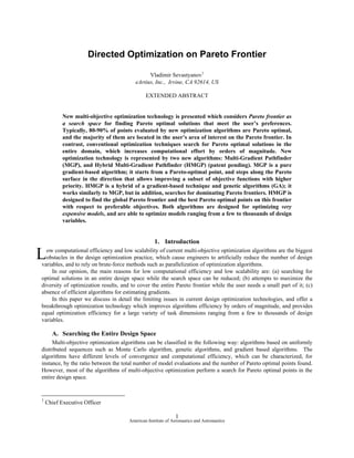
  • 20. FIG. 20A shows Pareto optimal points found by HMGP algorithm for the benchmark task (13). By the price of 600 evaluations HMGP found the exact global Pareto front, and covered the front completely. HMGP started from the blue initial point (see FIG.20A), and sequentially found several local Pareto frontiers. Fragments of local Pareto frontiers parallel to the green front can be seen on FIG. 20B in red. At the very end of the optimization session HMGP found the global Pareto frontier, and covered it from the beginning to the end. FIG.20B Results of HMGP after 400 evaluations, and results of Pointer after 1200 evaluations, NSGA-II and AMGA -- after 1500 evaluations. All points evaluated by each algorithm are visualized. HMGP has found and evenly covered global Pareto frontier. Pointer has found a few Pareto optimal points corresponding to low values of F1. NSGA-II and AMGA could not approach the global Pareto frontier after 1500 model evaluations. Benchmark problem ZDT3 with multiple disjoint Pareto frontiers The optimization task formulation used is as follows: 20 American Institute of Aeronautics and Astronautics
  • 21. Minimize F1 = x1 ⎡ F F ⎤ Minimize + F2 = g ⋅ ⎢1 − 1 − 1 sin(10 π F1 ) ⎥ ⎣ g g ⎦ (14) n 9 g = 1+ ∑ xi n − 1 i =2 0 ≤ xi ≤ 1, i = 1,..n; n = 30 FIG.21 Results of HMGP after 800 evaluations, and results of Pointer, NSGA-II and AMGA after 1500 evaluations. Only Pareto optimal points and 1st rank points are visualized on the charts. HMGP has found and covered all five disjoint segments of global Pareto frontier. Pointer has covered only three of five segments of the Pareto frontier. NSGA-II and AMGA were not able to approach the global Pareto frontier. The optimization results exposed on the diagrams FIG.19-FIG.21 confirm that HMGP algorithm consistently shows better efficiency and accuracy compared with Pointer, NSGA-II and AMGA optimization algorithms. 8. eArtius Design Optimization Tool eArtius has developed a commercial product Pareto Explorer, which is a multi-objective optimization and design environment combining a process integration platform with sophisticated, superior optimization algorithms, and powerful post-processing capabilities. Pareto Explorer 2010 implements the described above optimization algorithms, and provides a complete set of functionality necessary for a design optimization tool: • Intuitive and easy to use Graphical User Interface; advanced IDE paradigm similar to Microsoft Developer Studio 2010 (see FIG.22); • Interactive 2D/3D graphics based on OpenGL technology; • Graphical visualization of optimization process in real time; • Process integration functionality; • Statistical Analysis tools embedded in the system; • Design of Experiments techniques; • Response Surface Modeling; • Pre- and post-processing of design information; • Data import and export. 21 American Institute of Aeronautics and Astronautics
  • 22. All the diagrams included in this paper are generated by Pareto Explorer 2010. The diagrams give an idea about the quality of data visualization, the ability to compare different datasets, and a flexible control over the diagrams appearance. FIG. 22 shows a screenshot of Pareto Explorer main window. In addition to the design optimization environment implemented in Pareto Explorer, eArtius provides all the described algorithms as plug-ins for Noesis OPTIMUS, ESTECO modeFrontier, and Simulia Isight design optimization environments. Additional information about eArtius products and design optimization technology can be found at www.eartius.com. 9. Conclusion A new concept of directed optimization on Pareto frontier is introduced, and Multi-Gradient Pathfinder (MGP) algorithm is developed based on this concept. According to the concept, MGP performs optimization search directly on Pareto frontier in a preferred direction determined by the user’s preferences. This allows the following: (a) Avoiding a search in the areas that do not contain Pareto optimal points; as result, 80-95% of evaluated points are Pareto optimal; (b) Performing a search for the best optimal solutions only in the user’s area of interest and dramatically reducing computational effort; (c) Precise approachment to a desired solution on Pareto frontier instead of inaccurate approachment typical of GAs and other conventional optimization techniques. MGP has unparalleled efficiency because of the (a)-(c) reasons explained above, and also because of an increased control over the optimization process given to the user. For instance, MGP is able to perform a number of steps determined by the user, and then stop. In this mode, the user can precisely find a desirable improvement for the best known design by the price of just 10-15 evaluations! Thus, MGP can be used for optimization of extremely computationally expensive simulation models taking hours and even days for a single evaluation. Obviously, MGP 22 American Institute of Aeronautics and Astronautics
  • 23. is good for fast models as well. Hybrid Multi-Gradient Pathfinder (HMGP) algorithm is also developed based on the same concept of directed optimization on Pareto frontier. HMGP employs a gradient-based technique, and behaves similarly to MGP. But in addition, HMGP employs GA technique to search for dominating Pareto fronts. HMGP starts gradient-based steps along dominating Pareto front as soon as the first dominating Pareto optimal point is found by GA-based part of the algorithm. HMGP is very efficient in finding the global Pareto frontier, and in finding the best point on it with respect to preferable objectives. Both MGP and HMGP algorithms employ eArtius response surface method DDRSM [2], which allows efficient optimizing models with dozens and hundreds of design variables. Comparison of HMGP with state of the art commercial multi-objective optimization algorithms NSGA-II, AMGA, and Pointer on a number of challenging benchmarks has shown that HMGP finds global Pareto frontiers 2- 10 times faster. This allows to avoid using DOE and surrogate models for global approximation, and instead apply HMGP directly for the optimization of computationally expensive simulation models. HMGP is the best choice for solving global multi-objective optimization tasks for simulation models with moderate estimation time when 200-500 model evaluations are considered as a reasonable number of model evaluations for finding global Pareto optimal solutions. 10. References 1. Marler, R. T., and Arora, J. S. (2004), "Survey of Multi-objective Optimization Methods for Engineering", Structural and Multidisciplinary Optimization, 26, 6, 369-395. 2. Vladimir Sevastyanov, Oleg Shaposhnikov Gradient-based Methods for Multi-Objective Optimization. Patent Application Serial No. 11/116,503 filed April 28, 2005. 3. US Patent # 7,593,834, 2009. Lev Levitan, Vladimir Sevastyanov. The Exclusion of Regions Method for Multi- Objective Optimization. 4. Vanderplaats, Garret N. 1984. Numerical Optimization Techniques for Engineering Design: With Applications, McGraw Hill Series in Mechanical Engineering. 5. Bellman, R.E. 1957. Dynamic Programming. Princeton University Press, Princeton, NJ. 23 American Institute of Aeronautics and Astronautics