1. Issues and Policy Solutions to Commodity Price Volatility in the
European Union
Paper presented to the 2nd IFAMA Annual Symposium The Road to 2050. The China
Factor, Shanghai, June 2012
1,2
Monika Tothova, Beatriz Velazquez
European Commission
Directorate General for Agriculture and Rural Development
Abstract: Increased price levels – and related elevated price volatility – have been
discussed in the policy arena at least since the price hikes of 2007-08. While a number of
studies looked at volatility levels on the international markets, current paper looks in detail
on the EU and compares developments in price volatility on the EU and international
markets. As market environment is changing, policy is adjusting. The paper illustrates
instruments available to deal with volatility, indicating advantages and disadvantages based
on implementation experience. The role of market instruments as a product safety-net and
that of decoupled payments is to make farms less vulnerable to fluctuations in prices and to
provide an income safety net independent of the market situation. Current CAP instruments
need to be adjusted to achieve the objectives of market stability in light of the medium-term
market perspectives, in the most effective and efficient way. A concluding paragraph
indicates broadly what type of instruments could be suitable in a future CAP context.
1 Reasons to address volatility
Price levels and price volatility gained spotlight following the "food crises" in the late 2007
and early 2008 highlighting issues of food security and replacing previous concerns about
low commodity prices. Although price volatility is a normal feature of markets given the
seasonal production cycle and discontinuity of supply in the face of a continuing demand, a
greater uncertainty of rapidly changing economic and natural environments contributes to
and magnifies its occurrence.
The issue of volatility is central to today’s EU policy debate. The reason is twofold. On the
one hand, the medium-term perspectives for EU agricultural commodity prices are
expected to stay firm over the medium term, supported by factors such as the growth in
global food demand, the development of the biofuel sector and a prolongation of the long-
term decline in food crop productivity growth. High prices at world level would support
EU agricultural exports in spite of the decline in competitiveness, particularly with the
assumed appreciation of the EUR. But this market outlook faces a number of uncertainties
regarding future market developments as well as the macroeconomic and policy settings,
1 This paper is an updated and revised version of Tothova (2011), "Main Challenges of Price Volatility on
Agricultural Commodity Markets," and Velazquez (2011) "Dealing with Volatility in Agriculture: policy
issues" in Isabelle Piot-Lepetit and Robert M'Barek (editors), Methods to Analyze Agricultural Commodity
Price Volatility, Springer.
2 Corresponding author Beatriz.Velazquez@ec.europa.eu
Disclaimer: The views expressed in this chapter are those of the authors and should not be attributed to their
affiliated institution.

2. for example, the impact of a policy-driven slow down in economic growth in China in
order to curb price inflation or the impact of yield variations, e.g. due to weather
conditions, and the impact of increasing production costs in the EU. Other factors, such as
future changes in agricultural and trade policies, e.g. with a possible agreement within the
current Doha Development Round negotiations and/or in bilateral/regional trade
discussions, or renewable policies could have far reaching implications for the future
pattern of EU agricultural markets.
On the other hand, the move towards greater market orientation has exposed European
farmers to higher market volatility, and they are also more sensitive to changes in the
macroeconomic environment (like GDP and/or exchange rate fluctuations). Instability on
world commodity markets may also permeate to European Union (EU) markets as a
consequence of greater trade openness.
The fist part of this paper sets the scene for the policy discussion. It explores some
theoretical aspects of volatility and looks at increased volatility on international agricultural
commodity markets. Analysis focus on price developments on the EU and international
markets to identify whether one or another was more affected by increases in price
volatility. Based on previous analysis and on literature review, factors influencing price
volatility are illustrated in paragraph 3. The second part of this paper is devoted to the
possible role of policy instruments in dealing with volatility. It starts by presenting existing
and past policy instruments which have been used to deal with volatility (paragraph 4),
outlining their advantages and disadvantages, then it shows how volatility is currently dealt
with within the CAP. Based on experience from implementation, the concluding section
highlights implications from increased volatility, including suitable instruments in a future
context.
2 A close look at price volatility
Volatility provides a measure of the possible variation or movement in a particular
economic variable. Prices change as rapid adjustments to market circumstances. Wide price
movements over a short period of time typify the term "high volatility". What constitutes a
volatile market or an "excess volatility" can be subjective, sector and commodity specific.
While two measures of volatility – historical (realised) and implicit are used in the
literature, this paper focuses on historical price volatility which reflects the resolution of
supply and demand factors in the past. Historical volatility can also serve as an indicator of
the possible price changes of the assets – including commodities – in the future. Assets –
commodities including – that have high volatility are likely to undergo larger and more
frequent price changes in the future, possibly attracting market participants benefiting from
frequent price changes. Casual link between volatility and uncertainty is not clearly
defined: volatility thrives in the environment of uncertainty, and volatile prices themselves
contribute to uncertainty to producers, processors, and consumers.
2

3. 2.1 Has price volatility increased?
The G20 and other international discussions aim to discuss increased price volatility and
available policy options. The G20 report prepared by a group of international organisations
for the French presidency in 20113 states:
"When looked at in the long term there is little or no evidence that volatility in international
agricultural commodity prices, as measured using standard statistical measures is increasing and
this finding applies to both nominal and real prices5. Volatility has, however, been higher during the
decade since 2000 than during the previous two decades and this is also the case of wheat and rice
prices in the most recent years (2006-2010) compared to the nineteen seventies. Another conclusion
that emerges from the study of long term trends in volatility is that periods of high and volatile
prices are often followed by long periods of relatively low and stable prices. "
Many calculations of long term volatility rely on monthly data which are averages of more
variable higher frequency (often daily) data. Data with higher frequency exhibit higher
volatility. Volatility decreases with decreasing frequency. Cash (spot) prices such as c.i.f.
(cost, insurance, freight) can bring additional uncertainties to the analysis since transport
prices in their own are very variable, influencing the result. F.o.b. prices (free on board) are
better candidates for analysing volatility.
Commodity exchanges provide a steady stream of daily settlement prices making them
ideal for analysis. However, futures markets do not exist or are not used for all
commodities. In addition, some contracts may suffer from lack of convergence between
cash and future prices.
There might not be agreement on whether the price volatility of agricultural commodities
increased over the long run. While correct on the technical grounds, the findings are not of
immediate relevance to producers who were faced with lower price variability in the
preceding two decades. There seems to be an agreement that recent levels of price volatility
are rather high. In addition, what matters for producers and operators in business is whether
price volatility increased over the shorter period of time, and whether they have the
necessary tools and ability to confront it.
The analysis presented in the paper does not aim to analyse whether price volatility
increased in the long term. Rather, it compares price developments on the world and EU
markets using monthly data, and considers policy options in the EU.
2.2 An intuitive approach using spot prices
For illustrative purposes we used a simple coefficient of variation to describe price
variability from January 1998 to December 2011 to determine whether:
(1) world markets experienced higher price variation than EU markets
(2) price variation on international and EU commodity markets increased over time
3 http://www.oecd.org/dataoecd/40/34/48152638.pdf
3

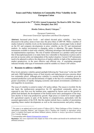
4. Figure 1 Monthly price developments on the EU internal market from January 1997 to
March 2012.
EU Market Prices for Representative Products
Cereals: euro/t, dairy and beef: euro/100 kg
450
400
350
300
250
200
150
100
Breadmaking wheat Feed maize SMP Butter Beef
50
0
ec ul 99
M r2 0
ec ul 04
M r2 5
ec ul 09
M r2 0
ov ne 97
pt pri 97
Fe be 998
r 9
O ay 99
ov ne 02
pt pri 02
br r 2 3
r 4
O ay 4
ov ne 07
pt pri 07
br r 2 8
r 9
O ay 9
12
7
ry 8
Au ch 00
Ja ust 01
2
ry 3
ch 05
Ja ust 06
7
ry 8
ch 10
Ja ust 11
ar 01
ar 06
ar 11
e 0
e 0
e 1
be 99
Fe be 00
be 00
M 200
Fe be 00
be 00
M 200
be 99
ua 99
be 00
ua 00
be 00
ua 00
ob 20
ob 20
ob 20
D J 19
D J 20
D J 20
N Ju 20
N Ju 20
N Ju 19
Se A r 19
M 19
Se A r 20
Se A r 20
20
g 20
ar 0
ar 0
g 20
ar 0
g 20
nu 20
nu 20
nu 20
em l 1
em y 1
em l 2
em y 2
em l 2
em y 2
em 1
br r 1
em 2
em 2
y
y
ry
y
a
nu
Au
Au
ct
ct
ct
Ja
Source: Agriview
EU data were taken from DG Agriculture EU market price datawarehouse (Agriview) for
representative products, and international commodity prices from international benchmarks
from the World Bank or FAO. Some commodities might not be directly comparable in
terms of quality and in some cases price data were not available on both world and the EU
markets. Data and sources are described in Annex 1.
A coefficient of variation is defined as a ratio of standard deviation over mean as a measure
of dispersion of data points. The higher is the coefficient of variation, the larger the
dispersion of series and higher the price volatility.
Table 1 shows coefficient of variations for comparable products on the world and EU
markets. Comparing coefficients of variation on the world and EU markets covering period
from January 1998 to December 2011 we observe that the prices on the world markets were
more dispersed than prices on the EU markets, with meats being less disperse than crops
and dairy. On both the world and EU markets the coefficient of variation increased between
1998 – 2004 and 2005 – 2011, indicating increased dispersion of prices. However, world
markets experienced more dispersed prices in the first period between 1998 and 2004 than
EU markets did. Even in the second time period the coefficient of variation in the world
price series exceeded the coefficient of variation in the EU.
4

5. Table 1 - Coefficient of variation, comparable products (%)
Commodity 1998- 1998-1- 2005-2011 1998- 1998- 2005-
2011 2004 2011 2004 2011
World prices EU prices
Barley 37.05 15.86 29.22 24.15 7.90 27.79
Wheat (SRW, EU bread) 42.26 17.70 32.14 25.30 8.65 29.60
Maize 44.21 12.08 35.88 22.45 9.31 26.17
Butter 47.97 19.47 34.55 11.53 3.54 15.74
SMP 39.85 18.96 31.46 14.33 8.44 17.74
Chicken 15.62 9.10 10.50 11.61 6.26 9.03
Beef 25.98 13.94 18.68 8.87 4.26 7.15
Price charts with trend lines for comparable products are presented in Annex 2. Note
different units: world prices are quoted in USD/t while European ones in euro.
Table 2 shows coefficient of variation for EU prices for which respective world equivalents
were not identified. The coefficient of variation increased significantly for crops and
cheeses while decreased for meats and remained relatively stable for eggs.
Table 2 - Coefficient of variation in EU prices: (%)
Commodity 1998-2011 1998-2004 2005-2011
Feed wheat 26.86 11.68 31.15
Durum wheat 34.58 11.28 36.88
Malting barley 26.69 7.62 28.32
Cheddar 17.62 6.17 14.44
Edam 9.18 5.88 10.69
Young bovines 10.53 6.94 6.36
Cows 10.81 7.62 5.60
Heifers 8.80 4.56 5.52
Piglets 18.18 22.82 12.28
Pork 12.18 15.19 7.44
Eggs 16.30 15.13 14.18
Preliminary conclusions can be drawn using the coefficient of variation: from January 1998
to December 2011 world commodity markets experienced more volatility than EU markets.
Coefficient of variation increased both on the world and EU markets between 01/1998 –
12/2004 and 01/2005 – 12/2011, with the EU often recording more dramatic increases.
However, in absolute terms the coefficient of variation in many cases remains higher on the
world than on the EU markets during 2004 – 2011.
2.3 Volatility on the futures markets
Commodity exchanges produce a stream of daily settlement data. The use of nearby futures
is also justified by frequently using nearby futures as international reference prices. The
CME Group offers already calculated measures of volatility4. For consistency in the case of
4 http://www.cmegroup.com/market-data/reports/historical-volatility.html. Data available up to August 2011.
To annualise their volatility figures, the CME group uses an average of 252 trading days each year. Due to
5

6. European exchanges we used settlement prices and formula applied in the CME
calculations for milling wheat (from September 1998 to March 2012) contract on MATIF.
The formula outlined in Annex 3.
Although different products on the CBOT (wheat, maize, oats, soybeans and derived
products) show different price and volatility patters, there are commonalities across them.
Although increased volatility can occur in any given period, actual peaks differ on the basis
of the commodity and developments of their fundamentals. Due to space limitation we
focus on wheat. Figure 2 shows historical volatility of wheat on CBOT on a monthly basis
from January 1980 to August 2011. Wheat volatility has had an increasing trend over the
observed period, ranging between 30 and 73. In the last four years the average volatility has
increased.
Figure 2 - CME Wheat Historical Volatility, monthly annualised
Wheat: CME Historical Volatility
monthly annualised
80
January 1980 - August 2011
70
60
50
Percent
40
30
20
10
0
80
81
82
83
84
85
86
87
88
89
90
91
92
93
94
95
96
97
98
99
00
01
02
03
04
05
06
07
08
09
10
11
19
19
19
19
19
19
19
19
19
19
19
19
19
19
19
19
19
19
19
19
20
20
20
20
20
20
20
20
20
20
20
20
Source: CME
Agricultural commodities traded on European exchanges, although smaller in terms of
volume, were not shielded from increased volatility. Figure 3 show the development of
historical volatility for milling wheat on MATIF.
holidays and weekends the number of actual trading days each year can differ, and as such volatility results
can differ.
6

7. Figure 3 - MATIF Milling Wheat, Historical Volatility, Monthly annualized
Wheat: MATIF Historical Volatility
monthly annualised
September 1998 - March 2012
80%
70%
60%
50%
Percent
40%
30%
20%
10%
0%
Se M ry 1 98
nu r 1 9
Se M ry 2 99
nu r 2 0
Se M y 2 0
nu r 2 1
Se M y 2 1
nu r 2 2
y 2
nu r 2 3
Se M y 2 3
nu r 2 4
y 4
nu r 2 5
Se M y 2 5
nu r 2 6
Se M ry 2 06
nu r 2 7
Se M y 2 7
nu r 2 8
Se M ry 2 08
nu r 2 9
Se M y 2 9
nu r 2 0
Se M y 2 0
nu r 2 1
y 1
em y 9
em y 0
em y 1
em y 2
em y 3
em y 4
em y 5
em y 6
em y 7
em y 8
em y 9
em y 0
em y 1
12
pt a 99
Ja be 99
pt a 00
Ja be 00
ar 00
pt a 00
Ja be 00
ar 00
pt a 00
Ja be 00
ar 00
pt a 00
Ja be 00
ar 00
pt a 00
Ja be 00
ar 00
pt a 00
Ja be 00
ar 00
pt a 00
Ja be 00
pt a 00
Ja be 00
ar 00
pt a 00
Ja be 00
pt a 00
Ja be 00
ar 00
pt a 01
Ja be 01
ar 01
pt a 01
Ja be 01
ar 01
a 9
a 9
a 0
a 0
20
1
2
2
2
2
2
2
2
2
2
2
2
2
nu r 1
Se M 2
Se M 2
J a be
em
pt
Se
Data source: MILLING WHEAT #2: 1ST EXPIRATION FUTURE NEARBY - SETL - MARCHE A TERME
INTERNATIONALE DE FRANCE (MATIF) via Global Insight. In-house calculations.
MATIF wheat experienced the highest volatility in September 2007, January 2009, and
July – August 2010 when it reached around 44 - 48 . The summer 2010 high volatility
episode accompanied poor harvest prospects in Russia and consequent export ban.
However, in between those peaks, the volatility was as low as 8 (February 2010).
Although experiencing peaks, wheat volatility on MATIF was relatively stable between
1998 and mid-2006 when it started increasing.
3 Factors influencing price volatility
Factors driving price volatility have been studied in detail during and following the price
hikes of 2007-2008 (e.g. EC, 2008; Meyers, 2009; Trostle, 2008; Baffes and Haniotis
2010). Among those underlying market fundamentals we can cite, among others, yields and
stock levels; weather and changing weather patterns with their related impacts; cycles in
key markets; policy driven developments including large purchases by the governments;
developments outside the agricultural sector such as exchange rate and oil price
movements; trade policies and their transmission; investment in agricultural production.
Commodities for which the demand is inelastic (such as agricultural products) tend to be
more volatile. Long-term structural changes are also responsible for the increase in price
variability, although their effects are not immediate. Only some of the factors contributing
to greater volatility are described below.
Low levels of stocks in their own right do not result in high price but provide in a limited
buffering capacity should increasing demand or short term supply challenges occur. There
is no single answer to the question of "what normal stocks are". In addition, stock
management, such as stock creation and release, can affect market fundamentals and
impact prices.
7

8. Climate change and weather related events impact production variability, and thus impact
market fundamentals. So far on the EU level, no correlation has been established between
the warming of the last decades and the level of crop yields, which have generally
increased (EC, 2009). However, impact of climate change might be already visible in other,
more vulnerable countries.
A frequent culprit of increased price volatility is "speculation" based on investing in
futures contracts on commodity markets to profit from price fluctuations. The wider and
more unpredictable price changes are, the greater the possibility of realizing large gains by
speculating on future price movements of the commodity in question. Although a presence
of "speculators" on the derivatives markets is a necessary condition for functioning markets
and efficient hedging, volatility can attract significant speculative activity and destabilise
markets, which are both the cause and effect of increased volatility. In thinly traded
markets where only small quantities of physical goods are traded, the value of speculative
trades may create false trends and drive up prices for consumers. Arguments both for (e.g.
Irwin and Sanders, 2010) and against (e.g. Robles et al, 2009) "speculation" are ample
although evidence is inconclusive. While other factors and fundamentals are at play and
have to be considered, there is a time overlap between increased volatility and increase in
open interests on the commodity markets. While increase in open interests and inflow of
investment money increases the liquidity on the market, increased liquidity could come
along with increased volatility.
Policies. Greater market orientation of agricultural policies (CAP including) relies on a
greater transmission of market signals, and results in more variable prices. Policy
instruments (described later) are in place to mitigate effects of price variability. Trade
restrictive policies also play a role in limiting supplies, thus increasing uncertainty on the
markets and price variability.
Strong co-movements with energy and other agricultural prices. Linkages with energy
markets before the emergence of biofuels were one-way: oil and energy as inputs to
agricultural production. Increased connection between energy and agriculture raises
questions about volatility transmission from more volatile energy and oil markets in
addition to changing market fundamentals, or at times without a significant change in
market fundamentals. The strength of the link is not yet determined, although Du et al
(2009) found evidence of volatility spill over among crude oil, maize, and wheat markets
after the autumn 2006 and explain it by tightened interdependence between these markets
induced by ethanol production.
Figures 4 and 5 show scatter chart of daily settlement data for maize and crude oil for
periods 2000-2004 and 2005-2010. An OLS line fitted to the data reveals stronger
correlation in the 2005-2010 time period with an R-squared of over 53 when not including
a trend variable, and 56 when including a trend variable to avoid spurious regression, with
all estimates significant at 5 level of significance. Scatter charts for data before 2000 (not
included) resemble that of 2000-2004, with no significant correlation.
8

9. Figure 4 - Scatter charts of maize and crude oil settlement prices, 2000 – 2004.
350
300
250
Maize settlement
200
150
100
50
0
0.00 10.00 20.00 30.00 40.00 50.00 60.00
Oil Settlement
Figure 5 - Scatter charts of maize and crude oil settlement prices, 2005 – 2010.
800
700
600
500
Maize settlement
400
300
200
100
0
0.00 20.00 40.00 60.00 80.00 100.00 120.00 140.00 160.00
Oil Settlement
4 Policy instruments to deal with volatility
There exist institutional reasons for addressing volatility, and they lie within the original
Common Agricultural Policy (CAP) objectives of stabilizing agricultural markets and
ensuring a fair standard of living for farmers from the Treaty of Rome. These objectives
have been left untouched by the Lisbon Treaty and thus remain valid for the future, but the
policy mix in place to achieve these objectives has been regularly adapted over the last
decades in line with a changing economic, social and political environment.
4.1 Price support
For a long time guaranteed institutional prices were the main tool within the CAP to ensure
support for farmers. Institutional prices set for agricultural products enabled domestic
prices to be kept relatively high and stable in comparison to those in the world market.
Moreover, in order to avoid increasing competition from imports, support prices had to be
accompanied by a certain degree of border protection (for example tariffs). If on the one
side EU markets were isolated − and thus protected − from external shocks, on the other,
9

10. high domestic prices boosted production, which in many cases exceeded domestic uses. As
a consequence, increasing amounts of production put market balances into risk (see Figure
6).
To re-establish equilibrium, quantities had to be withdrawn from the domestic market
through public intervention or exported to third countries. In such cases export refunds
were paid to bridge the gap between EU and world market prices. Increasing stocks
cumulated for many sectors (e.g. cereals, butter, wine). As a result, budgetary costs
increased steadily, leading to the budgetary crisis of the 1980s and the ensuing reform in
the mid-1990s.
Figure 6 - Price support
Prices
excess production
supply
PEU
P*
Pworld
demand
Quantities
Q* Q1
Through the various reforms (1992, 1999 and 2003), and with support switching from
product to producer support through decoupled payments, intervention systems have been
reviewed accordingly, with intervention prices being progressively reduced and aligned to
world prices. Public intervention today represents a targeted product safety-net (namely
private and public storage). Institutional prices are set at a level that ensures they are used
only in times of real crisis. However, intervention is justified under conditions of force
majeure (e.g. extreme weather) to compensate farmers for high income variability due to
extreme variations in prices (e.g. Arts 70-71 of Reg. 73/2009 on direct payments).
4.2 Supply control
Quantitative restrictions, for example sugar and dairy quotas, had to be introduced in order
to deal with market imbalances − including those created by high price support − as well as
to contain budgetary costs.
Although it is true that in period of over-production quotas contributed to reduce budgetary
costs and to improve market balance, the rigidity they create has detrimental effects on
price stability. The impact on prices of any shock on the demand (or supply) side is swelled
by the fact that supply cannot adapt to these changes (see Figure 7). This drawback is of
particular importance for agricultural markets.
10

11. Figure 7 - Quotas
Prices
supply
Price1
∆P1
Price*
demand2
∆P2
Price2 demand
demand1
Quantities
quota
The recent dairy crisis provides a good example. Agricultural prices declined sharply from
September 2008 until May 2009 following the demand drop resulting from the economic
crisis and dairy farmers suffered more than other actors in the dairy food chain. This can be
explained mainly by the rigidity of the sector, in particular by constraints hampering supply
response to price signals.
Other factors played a part as well, among them a low price transmission along the food
chain, lack of transparency, and lower bargaining power with respect to other actors in the
chain. These elements have been examined by the dairy High Level expert Group on milk
(HLG) of experts, which in its final report (European Commission, 2010) identified, in
contractual and inter-professional arrangements, a way to increase the bargaining power of
farmers and to improve the food chain organization.
4.3 Stability through price guarantee – counter cyclical payments
Counter cyclical payments are implemented in the United States. They have been designed
to support and stabilize product-specific revenue, and indirectly income, in years when
current prices for historically produced commodities are lower than target prices (Dismukes
and Coble 2007). Thus, when market prices fall, payments increase. These programmes
provide a payment when the actual price falls below a certain reference level, protecting
farmers against price risks. A farmer gets no compensation through this scheme for low
yields, as the price compensation is only paid for the actual yield.
Counter cyclical payments have several major drawbacks. The unpredictability of
budgetary expenditures and insulation of farmers from market signals are two of the best
known. They are also problematic from a WTO point of view as they are linked to current
prices, and thus trade distorting.
The biggest drawback is the lack of any link to real farm income, since they do not take
into account the total yield and the farm cost of production. When the yield is low, or when
input costs increase but the market price of the related crops does not increase
proportionally, the programme fails to deliver its targeted aim - it guarantees price for a
specific crop but not income.
11

12. Figure 8 below shows how counter cyclical payments work in the US model, introduced as
an additional safety-net to the Loan Payments Programme by making up the difference
between low commodity prices and pre-determined target prices.
Figure 8 - Counter cyclical payments
Price/mt
Market price
Target price
Loan rate
Loan payments Counter cyclical payments Target price Loan rate Market price
4.4 Stability through decoupled support
Decoupled direct payments have been introduced with the 2003 CAP reform. They can be
seen as a way to stabilize and enhance farm income by guaranteeing a basic fixed income
support to farmers and as such representing a producer safety-net. This is illustrated in
Figure 9, where real prices and revenues per hectare in the EU during the last thirty years
are put together with the EU average value of direct payments.
This type of income stabilization through direct payments makes farms less vulnerable to
fluctuations in prices providing an income safety net independent of the market situation.
Without such stabilization many farms, including economically viable enterprises that
could potentially respond to the long-term demands of the sector, may come under threat
and could be forced out of business. Reducing the income variability gives these farms the
necessary liquidity to survive crises, reduces investment risks, and, thereby, contributes to
maintain economically sound farms in the sector in the long run.
Results from simulations (ECNC, LEI, ZALF 2009) showed that a sudden termination of
direct payments would lead to disruptive income losses that could force a large number of
farmers out of the sector. This supports the idea that income support smoothes out the
structural adjustment process and allows a gradual adaptation of the sector and the rural
areas to the new conditions, avoiding disruption to existing structures.
12

13. Figure 9 -Decoupled support
300 1 5 00
250 1 2 5 0
200 1 000
150 7 5 0
100 5 00
50 2 5 0
0 0
M a rk e t p ric e s R e v e n u e /h a D ire c t p a y m e n ts
4.5 Stability through income guarantee
In the EU the idea of an income stabilization tool has been floating since the 2003 CAP
reform. One option put forward in the 2005 Communication on risk and crisis management
in agriculture examined an income stabilization tool. Under this option farmers would be
compensated for a serious fall in income, in particular a fall of more than 30%.
The Commission5 made an analysis of the income stabilization tool using FADN data for
EU25 in the period 1998-2007. The farm net value added (FNVA) was used as income
indicator. Estimates have been calculated on the share (%) of farms that would be eligible
for compensation, and the budget needed for EU25 in the period 1998-2007 (see Figure
10).
5 Directorate for Agriculture estimates calculated using FADN data.
13

14. Figure 10 - Income Stabilization tool: Share of farms eligible for compensation, and
compensation need over time
Bio EUR of % of farms
compensation
18 30
15 25
12 20
9 15
6 10
3 5
0 0
1998 1999 2000 2001 2002 2003 2004 2005 2006 2007
Compensation EU-15 Compensation EU-9 % of farms EU-15 % of farms EU-9
Note: Gross Farm Income used as income indicator; Average yearly compensation for EU-
15 for 1998-2007, for EU-10 (without Malta= EU-9) average 2006-07
Source: European Commission – DG Agriculture and Rural Development (FADN data)
As can be seen in the graph, the implementation of this instrument may be subject to a high
yearly variability in terms of expenditure, which may also have an impact on potential
recipients in terms of production behaviour. Other challenges for applying an income
stabilization tool at EU level are related to budgetary needs - this tool would require on
average approximately 10 billion Euros per year for EU25 - also the organizational
arrangements could also be complex to implement, both at EU and MS levels. Certainly,
these challenges invite the comparison between such a scheme and decoupled support in
terms of transfer efficiency.
A series of other questions needs to be addressed on its implementation: should it be an
EU-wide tool or a more targeted one, articulated according to different situations across the
EU and across sectors?; should it be fixed or variable (for example like a top-up to
compensate income variability)?; should it be financed exclusively by the EU or also by
MS' own money?
4.6 Improving the food chain
The improvement of the functioning of the whole supply chain could be seen as an
alternative way to address the issue of volatility because it may contribute to market
stability. This is possible improving transparency and allowing an efficient price discovery
along the supply chain.
Figure 11 illustrates how price transmission along the food chain is channelled through the
different actors. Using price indexes (January 2007=100) it exclusively shows variations in
14

15. the recent past. It should be noticed that after a steep positive trend, commodity prices at
farm level already started a downward trend in February 2008, but prices paid by the
industry and retailers showed a lag of 6 and 12-18 months respectively. These time lags
indicate that during the crisis period farmers were the actors along the food chain to have
suffered most the price crisis since its very beginning.
Figure 11 - Short-term price evolution along the food supply chain
125
Agricultural
120 Commodity Prices
Food Producer Food Consumer
115
Prices Prices
110
Overall
inflation
105
100
95
20 /01
20 /03
20 /05
20 /07
20 /09
20 /11
20 /01
20 /03
20 /05
20 /07
20 /09
20 /11
20 /01
20 /03
20 /05
20 /07
20 /09
20 /11
20 /01
20 /03
20 /05
20 /07
20 /09
20 /11
20 /01
20 /03
20 /05
20 /07
20 /09
20 /11
20 /01
3
/0
07
07
07
07
07
07
08
08
08
08
08
08
09
09
09
09
09
09
10
10
10
10
10
10
11
11
11
11
11
11
12
12
20
Source: European Commission, based on Eurostat (Food Supply Chain Monitor) and DG Agriculture and Rural Development data
These instruments have been successfully implemented in certain sectors (fruit and
vegetables and wine) for a long time. In particular, measures aiming to promote the
creation of farmer producer organizations (POs), inter-branch organizations (IBOs), as well
as co-financing operational programmes. A series of competition rule derogations are
granted. Such instruments tend to have strong sector-specific characteristics, reflecting the
structure of the industry.
5 Volatility and the CAP of today
The core element of the latest CAP reform process has been the greater emphasis placed on
competitiveness and market orientation, with a decline in support for products and their
prices in favour of support for producers and their income. Effectively, it meant the
separation of the income support component (through de-coupled payment) from the
market stabilization component (through intervention). Intervention became less relevant
with the increased role of world markets, flexibility in farmers’ production choices, and
changes in supply chains and demand patterns. In this context, market stability is ensured,
allowing the efficient functioning of markets, stimulating its development and transparency
and facilitating participation of actors. The reform process also implied a move from
policies concentrated mostly on commodity markets to horizontal instruments, which can
benefit differentiated niche markets and a wide range of market actors.
15

16. Historical trends in EU prices highlight the results of this market orientation process. In
most commodities, EU market prices have been decreasing over 1991-2011 and today they
are close to world prices.
Figure 12 - Reductions in EU price support, bringing EU prices in line with world prices
0%
-10%
-20%
-30%
-40%
-50%
-60%
-70%
In nominal terms In real terms
-80%
-90%
-100%
Soft wheat Beef Butter SMP White sugar
Source: European Commission - DG Agriculture and Rural Development
In the same fashion, trends in EU prices for most commodities mirror those of world prices
because markets are much more connected, but this higher “exposure” to market changes
and trends increased beyond what was previously foreseen. This was obvious during the
commodity price boom in 2007 and then during the price slow-down that followed the
economic crisis in 2009. On both occasions prices showed a historically high volatility,
with very sharp variations in short periods of time.
From the perspective of increased price volatility and climate change, active risk
management will be increasingly important for farmers. There are several tools in the CAP
that address risks that farmers face. Firstly, there exists the possibility of subsidies for
farmers that subscribe to crop, animal and plant insurance against adverse climatic events,
and animal and plant diseases, creating mutual funds for combating animal and plant
diseases, and environmental incidents. Secondly, there are special risk and crisis
management measures for fruit and vegetables and wine: supporting (through producer
organizations or national envelopes) production planning; concentration of supply;
promotion of products; green harvesting; non-harvesting, harvest insurance, market
withdrawals, free distribution, promotion and communication, mutual funds, potable
alcohol distillation, crisis distillation, by-product distillation. Lastly, two measures address
production risks among those of a Rural Development toolkit: introducing appropriate
prevention measures against natural disasters in agriculture and forestry; and restoring
agricultural and forestry production potential damaged by natural disaster (Measure 126
and 226) , and “Vocational training and information”, where risk management could be
addressed as one topic (Measure 111).
16

17. Based on what has been examined in preceding paragraphs, we can assert that thanks to
progressive reduction of support prices, intervention systems today represent a targeted
product safety-net, which is triggered only in exceptional circumstances and is no longer a
structural outlet for farmers (e.g. dairy crisis experience). However, there is still room for
improvement of the various intervention systems in place, to render them more efficient,
and easy to implement promptly and control in case of crisis.
Other instruments may complement intervention since they address sources of uncertainties
and farm income variability, such as farmers' low bargaining power and transparency.
Decoupled direct support, which constitutes the bulk of our agricultural support, provides a
producer safety-net to farmers, which is essential for farm economic viability. Effectively,
it contributes to ensure a certain farm income stability which, in combination with cross-
compliance, promotes sustainable farming activity.
6 Concluding remarks
Although references are often made to "excess volatility", it is generally accepted that a
certain degree of volatility is desirable, and price volatility is a normal feature of the
markets. Without price adjustments, markets would come to a stall. Volatility across the
commodity markets is not consistent. Although active participants on agricultural
commodity markets are finding prices to be volatile, compared to energy market, volatility
remains rather low. Energy returns have been significantly more volatile than other
commodity sectors. Other markets, such as metals, have experienced higher volatility than
energy markets; these episodes have been brief and transitory.
In macroeconomic terms, while price hikes are beneficial for net exporting countries that
benefit from improved balance of payments, they increase the import bill of net importing
countries.
Food security considerations play an important role. Variable prices lead to an uncertain
food import bill, and high prices impact the ability of poor consumers to purchase
necessary food. On the other hand, producers and net sellers benefit from increased prices.
Concerns about increased price volatility are usually voiced by producers and processors
who, in the absence of risk management tools, are exposed to unpredictability and
uncertainty associated with changing prices. High fluctuations in prices may limit the
ability of consumers (processors) to secure supplies and control input costs. Due to price
transmission issues, contracting and relatively low percentage of raw commodity in the
processed products, consumer prices do not necessarily follow commodity prices directly.
While we focus on the volatility of output prices, volatility of input prices (oil, fertilizer,
etc) also affects agricultural production and decision making.
The biggest drawback of volatility is the associated uncertainty of marketing production,
investment in technology, innovation, etc. The persistence in volatility reflects the
continued uncertainty in how market fundamentals have unfolded and how they are likely
to unfold this to go together with effects of volatility. Higher price volatility means higher
costs of managing risks (such as higher margins on futures contracts and higher premiums
for crop revenue insurance). It is likely that higher cost of risk mitigation would eventually
translate into higher consumer prices. Commodity shocks in the form of increased prices
17

18. and increased volatility can also have impact on inflation, although this article abstains
from analysing the link.
A distinction has to be made between the effects of volatility itself (such as unstable prices
and their impact on food security) and effects of policy reactions. Short term policy
reaction can contribute to market instability and consequently volatility, as we observed in
the case of rice in spring 2008 when in the wake of increasing price levels some major
exporting countries introduced export restrictions, and again in summer 2010 following an
export ban in Russia.
The EU past experience of implementing tools that tried to stabilise market using price or
supply controls has proved inadequate to today's context. The pressure on agricultural
income is expected to continue as farmers are facing more risks, a slowdown in
productivity and margin squeeze due to rising international prices. There is therefore a need
to maintain income support and to reinforce instruments to better manage risks and respond
to crisis situations.
The European Commission has tabled a set of proposals for reforming the CAP in October
2011 (EC, 2011, 2011a, 2011b), based on the Communication on the CAP towards 2020
(EC, 2010) that outlined broad policy options in order to respond to the future challenges
for agriculture and rural areas. Some of the proposed policy changes represent themselves
policy solutions to the issue of volatility:
• Measures for improving the food chain functioning and transparency, e.g. the
expansion of product coverage for the recognition of producer organisations and their
associations, and basic conditions if Member States make written contracts compulsory,
with a view to strengthening the bargaining power of milk producers in the food chain.
• A risk management toolkit including support to mutual funds and a new income
stabilization tool offers new possibilities to deal with the strong volatility in agricultural
markets that is expected to continue in the medium term.
• Changes in the way decoupled income support is granted to farmers, briefly:
• A single scheme across the EU, the basic payment scheme, replaces the Single
Payment Scheme and the Single Area Payment Scheme as from 2014. The
scheme will operate on the basis of payment entitlements allocated at national
or regional level to all farmers according to their eligible hectares in the first
year of application. Thus the use of the regional model that was optional in the
current period is generalized, also effectively bringing all agricultural land into
the system.
• With a view to a more equitable distribution of support, the value of
entitlements should converge at national or regional level towards a uniform
value. This is done progressively to avoid major disruptions.
• An important element is to enhance the overall environmental performance of
the CAP through the greening of direct payments by means of certain
agricultural practices beneficial for the climate and the environment that all
farmers will have to follow, which go beyond cross compliance and are in turn
the basis for rural development measures.
18

19. 7 References
Baffes J., Haniotis T. (2010). Placing the recent commodity boom in perspective. Policy
Research Working Paper 5371. The International Bank for Reconstruction and
Development/The World Bank, June 2010.
Dismukes R., Coble K.H. (2007). Managing risk with revenue insurance, USDA, ERS,
Amber Waves, 5 (Special Issue: May).
CNC-European Centre for Nature Conservation, Landbouw-Economisch Instituut (LEI)
and Leibniz-Zentrum für Agrarlandschaftsforschung e.V. (ZALF) (2009). Update of
analysis of prospects in the Scenar 2020 study. Preparing for change. Document
commissioned by the European Commission. Downloadable at.
http://ec.europa.eu/agriculture/analysis/external/scenar2020ii/index_en.htm.
European Commission, Directorate for Agriculture and Rural Development (2011).
Proposal for a Regulation of the European Parliament and of the Council establishing
rules for direct payments to farmers under support schemes within the framework of the
common agricultural policy, SEC(2011) 1153,1154. http://ec.europa.eu/agriculture/cap-
post-2013/legal-proposals/com625/625_en.pdf
European Commission, Directorate for Agriculture and Rural Development (2011a).
Proposal for a Regulation of the European Parliament and of the Council on support for
rural development by the European Agricultural Fund for Rural Development (EAFRD)
,SEC(2011) 1153, 1154 http://ec.europa.eu/agriculture/cap-post-2013/legal-
proposals/com627/627_en.pdf
European Commission, Directorate for Agriculture and Rural Development (2011b).
Proposal for a Regulation of the European Parliament and of the Council establishing
rules for establishing a common organisation of the markets in agricultural products
(Single CMO Regulation), SEC(2011) 1153, 1154. http://ec.europa.eu/agriculture/cap-
post-2013/legal-proposals/com626/626_en.pdf
European Commission, Directorate for Agriculture and Rural Development (2010). Report
of the high level group on milk.
http://ec.europa.eu/agriculture/markets/milk/hlg/report_150610_en.pdf
European Commission, Directorate for Agriculture and Rural Development (2010a).
Communication from the Commission to the European Parliament, the Council, the
European Economic and Social Committee and the Committee of the Regions The CAP
towards 2020: meeting the food, natural resources and territorial challenges of the
future, COM(2010)672 final, 18.11.2010. http://eur-
lex.europa.eu/LexUriServ/LexUriServ.do?uri=COM:2010:0672:FIN:en:PDF
European Commission, Directorate for Agriculture and Rural Development (2008). Impact
assessment of the CAP Health Check. Commission staff working document, SEC(2008)
1885. http://ec.europa.eu/agriculture/healthcheck/fullimpact_en.pdf.
19

20. EC, 2008. High prices on agricultural commodity markets: situation and prospects.
Brussels. Available at:
http://ec.europa.eu/agriculture/analysis/tradepol/commodityprices/high_prices_en.pdf
EC, 2009. Commission Staff Working Document: Adapting to climate change: the
challenge for European agriculture and rural areas. SEC(2009) 147. Available at
http://ec.europa.eu/agriculture/climate_change/workdoc2009_en.pdf
Irwin, S. H. and D. R. Sanders (2010), “The Impact of Index and Swap Funds on
Commodity Futures Markets: Preliminary Results”, OECD Food, Agriculture and
Fisheries Working Papers, No. 27, OECD Publishing. doi: 10.1787/5kmd40wl1t5f-en
OECD
Meyers, William H. and Seth Meyer, 2009. Causes and Implications of the Food Price Surge,
Columbia, MO. Available at
http://www.fapri.missouri.edu/outreach/publications/2008/FAPRI_MU_Report_12_08.pdf
OECD, 2010. OECD – FAO Agricultural Outlook 2010. Paris.
Robles, Miguel; Maximo Torero and Joachim von Braun, 2009. When speculation matters,
IFPRI. Available at http://www.ifpri.org/sites/default/files/publications/ib57.pdf.
Trostle, Ronald, 2008. Global Agricultural Supply and Demand: Factors Contributing to
the Recent Increase in Food Commodity Prices, Washington DC. Available at
http://www.ers.usda.gov/Publications/WRS0801/
20

21. Annex 1: Description of the price series used
World grains, oilseeds and meats: compilation of various sources by World Bank
Commodity Price Data (Pink Sheet), available at http://go.worldbank.org/2O4NGVQC00
Barley (Canada), feed, Western No. 1, Winnipeg Commodity Exchange, spot, wholesale
farmers' price
Wheat (US), no. 2, soft red winter, export price delivered at the US Gulf port for prompt
or 30 days shipment
Maize (US), no. 2, yellow, f.o.b. US Gulf ports
Wheat (US), no. 1, hard red winter, ordinary protein, export price delivered at the US
Gulf port for prompt or 30 days shipment
Rice (Thailand), 5 broken, white rice (WR), milled, indicative price based on weekly
surveys of export transactions, government standard, f.o.b. Bangkok
Sorghum (US), no. 2 milo yellow, f.o.b. Gulf ports
Soybeans (US), c.i.f. Rotterdam
Soybean oil (Any origin), crude, f.o.b. ex-mill Netherlands
Soybean meal (any origin), Argentine 45/46 extraction, c.i.f. Rotterdam beginning 1990;
previously US 44
Meat, beef (Australia/New Zealand), chucks and cow forequarters, frozen boneless, 85
chemical lean, c.i.f. U.S. port (East Coast), ex-dock, beginning November 2002; previously
cow forequarters
Meat, chicken (US), broiler/fryer, whole birds, 2-1/2 to 3 pounds, USDA grade "A", ice-
packed, Georgia Dock preliminary weighted average, wholesale
World dairy prices: FAO compilation of average of mid-point of price ranges reported
bi-weekly by Dairy Market News (USDA). Available at
http://www.fao.org/es/esc/prices/PricesServlet.jsp?lang=en
Butter, Oceania, indicative export prices, f.o.b.
Cheddar Cheese, Oceania, indicative export prices, f.o.b.
Skim Milk Powder, Oceania, indicative export prices, f.o.b.
Whole Milk Powder, Oceania, indicative export prices, f.o.b.
EU market prices for representative products (monthly) Available at
http://ec.europa.eu/agriculture/markets/
21

22. USD/t
Ja
nu
ar
y
World
Barley
N Ju 19
0
50
100
150
200
250
300
ov n 9
em e 1 7
be 99
Se A r 1 7
pt pr 997
em il
Fe be 199
br r 1 8
ua 9
ry 98
D 1
ec Ju 99
em ly 1 9
be 99
r1 9
M
O ay 999
ct
ob 20
0
M er 2 0
ar 0
Au ch 00
g 2
Ja us 001
nu t 2
ar 00
y 1
N Ju 20
ov n 0
em e 2 2
be 00
Se A r 2 2
pt pr 002
em il
Fe be 200
br r 2 3
ua 0
ry 03
D 2
ec Ju 00
em ly 2 4
be 00
r 4
M 2
O ay 004
ct
ob 20
M er 05
ar 20
Barley, feed, spot, Canadian
Au ch 05
g 2
Ja us 006
nu t 2
ar 00
y 6
N Ju 20
ov n 0
em e 2 7
be 00
Se A r 2 7
pt pr 007
em il 2
Fe be 00
br r 2 8
ua 0
ry 08
D 2
ec Ju 00
em ly 2 9
be 00
r2 9
M
O ay 009
ct
ob 20
1
M er 2 0
ar 0
Au ch 10
gu 20
Ja s 11
Data Source: WB
nu t 2
ar 01
y 1
20
12
eur/t
EU
Ja
nu
ar
y
N Ju 19
0
50
100
150
200
250
ov n 9
em e 1 7
be 99
Se A r 1 7
pt pr 997
em il
Fe be 199
br r 1 8
ua 9
ry 98
D 1
ec Ju 99
em ly 1 9
be 99
r1 9
M
O ay 999
Annex 2 - Price charts with trend lines in prices of comparable products
ct
ob 20
0
M er 2 0
ar 0
Au ch 00
gu 20
Ja s 01
nu t 2
ar 00
y 1
N Ju 20
ov n 0
em e 2 2
be 00
Se A r 2 2
pt pr 002
em il
Fe be 200
br r 2 3
ua 0
ry 03
D 2
ec Ju 00
em ly 2 4
be 00
r2 4
M
O ay 004
ct
ob 20
0
M er 2 5
ar 0
Feed barley EU market price
Au ch 05
g 20
Ja us 06
nu t 2
ar 00
y 6
N Ju 20
ov n 0
em e 2 7
be 00
Se A r 2 7
pt pr 007
em il
Fe be 200
br r 2 8
ua 0
ry 08
D 2
ec Ju 00
em ly 2 9
be 00
r 9
M 2
O ay 009
ct
ob 20
M er 10
ar 20
Au ch 10
g 2
Ja us 011
nu t 2
ar 01
y 1
20
12
Data Source: AGRIVIEW