1. S UBMITTED : D ECEMBER 7, 2009; ACCEPTED : A PRIL 13, 2010
Preprint typeset using LTEX style emulateapj v. 2/16/10
A
SLOAN LOW-MASS WIDE PAIRS OF KINEMATICALLY EQUIVALENT STARS (SLoWPoKES):
A CATALOG OF VERY WIDE, LOW-MASS PAIRS
S AURAV D HITAL 1 , A NDREW A. W EST 2,3 , K EIVAN G. S TASSUN 1,4 , J OHN J. B OCHANSKI 3
Submitted: December 7, 2009; Accepted: April 13, 2010
ABSTRACT
We present the Sloan Low-mass Wide Pairs of Kinematically Equivalent Stars (SLoWPoKES), a catalog of
1342 very-wide (projected separation 500 AU), low-mass (at least one mid-K – mid-M dwarf component)
common proper motion pairs identified from astrometry, photometry, and proper motions in the Sloan Digital
Sky Survey. A Monte Carlo based Galactic model is constructed to assess the probability of chance alignment
for each pair; only pairs with a probability of chance alignment ≤ 0.05 are included in the catalog. The
overall fidelity of the catalog is expected to be 98.35%. The selection algorithm is purposely exclusive to
ensure that the resulting catalog is efficient for follow-up studies of low-mass pairs. The SLoWPoKES catalog
is the largest sample of wide, low-mass pairs to date and is intended as an ongoing community resource for
detailed study of bona fide systems. Here we summarize the general characteristics of the SLoWPoKES sample
and present preliminary results describing the properties of wide, low-mass pairs. While the majority of the
identified pairs are disk dwarfs, there are 70 halo subdwarf pairs and 21 white dwarf–disk dwarf pairs, as well
as four triples. Most SLoWPoKES pairs violate the previously defined empirical limits for maximum angular
separation or binding energies. However, they are well within the theoretical limits and should prove very
useful in putting firm constraints on the maximum size of binary systems and on different formation scenarios.
We find a lower limit to the wide binary frequency for the mid-K – mid-M spectral types that constitute our
sample to be 1.1%. This frequency decreases as a function of Galactic height, indicating a time evolution of
the wide binary frequency. In addition, the semi-major axes of the SLoWPoKES systems exhibit a distinctly
bimodal distribution, with a break at separations around 0.1 pc that is also manifested in the system binding
energy. Comparing with theoretical predictions for the disruption of binary systems with time, we conclude
that the SLoWPoKES sample comprises two populations of wide binaries: an “old” population of tightly bound
systems, and a “young” population of weakly bound systems that will not survive more than a few Gyr. The
SLoWPoKES catalog and future ancillary data are publicly available on the world wide web for utilization by
the astronomy community.
Subject headings: binaries: general — binaries: visual — stars: late-type — stars: low-mass, brown dwarfs —
stars: statistics — subdwarfs — white dwarfs
1. INTRODUCTION tute ∼70% of Milky Way’s stellar population (Miller & Scalo
The formation and evolution of binary stars remains one of 1979; Henry et al. 1999; Reid et al. 2002; Bochanski et al.
the key unanswered questions in stellar astronomy. As most 2010, hereafter B10) and significantly influence its properties.
stars are thought to form in multiple systems, and with the Since the pioneering study of Heintz (1969), binarity
possibility that binaries may host exoplanet systems, these has been observed to decrease as a function of mass: the
questions are of even more importance. While accurate mea- fraction of primaries with companions drops from 75%
surements of the fundamental properties of binary systems for OB stars in clusters (Gies 1987; Mason et al. 1998,
provide constraints on evolutionary models (e.g. Stassun et al. 2009) to ∼60% for solar-mass stars (Abt & Levy 1976,
2007), knowing the binary frequency, as well as the distribu- DM91, Halbwachs et al. 2003) to ∼30–40% for M dwarfs
tion of the periods, separations, mass ratios, and eccentrici- (Fischer & Marcy 1992, hereafter FM92; Henry & McCarthy
ties of a large ensemble of binary systems are critical to un- 1993; Reid & Gizis 1997; Delfosse et al. 2004) to ∼15%
derstanding binary formation (Goodwin et al. 2007, and refer- for brown dwarfs (BDs; Bouy et al. 2003; Close et al. 2003;
ences therein). To date, multiplicity has been most extensively Gizis et al. 2003; Mart´n et al. 2003). This decrease in bi-
ı
studied for the relatively bright high- and solar-mass local narity with mass is probably a result of preferential de-
field populations (e.g. Duquennoy & Mayor 1991, hereafter struction of lower binding energy systems over time by dy-
DM91). Similar studies of low-mass M and L dwarfs have namical interactions with other stars and molecular clouds,
been limited by the lack of statistically significant samples rather than a true representation of the multiplicity at birth
due to their intrinsic faintness. However, M dwarfs consti- (Goodwin & Kroupa 2005). In addition to having a smaller
total mass, lower-mass stars have longer main-sequence (MS)
1 Department of Physics & Astronomy, Vanderbilt University, 6301 lifetimes (Laughlin, Bodenheimer, & Adams 1997) and, as
Stevenson Center, Nashville, TN, 37235; saurav.dhital@vanderbilt.edu an ensemble, have lived longer and been more affected by
2 Department of Astronomy, Boston University, 725 Commonwealth Av-
dynamical interactions. Hence, they are more susceptible
enue, Boston, MA 02215
3 Kavli Institute for Astrophysics and Space Research, Massachusetts In- to disruption over their lifetime. Studies of young stellar
stitute of Technology, Building 37, 77 Massachusetts Avenue, Cambridge, populations (e.g. in Taurus, Ophiucus, Chameleon) appear
MA, 02139 to support this argument, as their multiplicity is twice as
4 Department of Physics, Fisk University, 1000 17th Ave. N., Nashville,
high as that in the field (Leinert et al. 1993; Ghez et al. 1997;
TN 37208

2. 2 Dhital et al.
Kohler & Leinert 1998). However, in denser star-forming re- the above, one can use additional information such as
gions in the Orion Nebula Cluster and IC 348, where more proper motions. Orbital motions for wide systems are
dynamical interactions are expected, the multiplicity is com- small; hence, the space velocities of a gravitationally
parable to the field (Simon, Close, & Beck 1999; Petr et al. bound pair should be the same, within some uncer-
1998; Duchˆ ne, Bouvier, & Simon 1999). Hence, preferen-
e tainty. In the absence of radial velocities, which are
tial destruction is likely to play an important role in the evo- very hard to obtain for a very large number of field stars,
lution of binary systems. proper motion alone can be used to identify binary sys-
DM91 found that the physical separation of the binaries tems; the resulting pairs are known as common proper-
could be described by a log-normal distribution, with the peak motion (CPM) doubles. Luyten (1979, 1988) pioneered
at a ∼30 AU and σlog a ∼1.5 for F and G dwarfs in the lo- this technique in his surveys of Schmidt telescope
cal neighborhood. The M dwarfs in the local 20-pc sample plates using a blink microscope and detected more than
of FM92 seem to follow a similar distribution with a peak at 6000 wide CPM doubles with µ >100 mas yr−1 over
a ∼3–30 AU, a result severely limited by the small number of almost fifty years. This method has since been used
binaries in the sample. to find CPM doubles in the AGK 3 stars by Halbwachs
Importantly, both of these results suggest the existence (1986), in the revised New Luyten Two-Tenths (rNLTT;
of very wide systems, separated in some cases by more Salim & Gould 2003) catalog by Chanam´ & Goulde
than a parsec. Among the nearby (d < 100 pc) solar- (2004), and among the Hipparcos stars in the Lepine-
type stars in the Hipparcos catalog, L´ pine & Bongiorno
e Shara Proper Motion-North (LSPM-N; L´ pine & Shara
e
(2007) found that 9.5% have companions with projected or- 2005) catalog by L´ pine & Bongiorno (2007). All
e
bital separations s > 1000 AU. However, we do not have of these studies use magnitude-limited high proper-
a firm handle on the widest binary that can be formed motion catalogs and, thus, select mostly nearby stars.
or on how they are affected by localized Galactic poten-
tials as they traverse the Galaxy. Hence, a sample of More recently, Sesar, Ivezi´ , & Juri´ (2008, hereafter
c c
wide binaries, especially one that spans a large range of SIJ08) searched the SDSS Data Release Six (DR6;
heliocentric distances, would help in (i) putting empirical Adelman-McCarthy et al. 2008) for CPM binaries with angu-
constraints on the widest binary systems in the field (e.g. lar separations up to 30 using a novel statistical technique
Reid et al. 2001a; Burgasser et al. 2003, 2007; Close et al. that minimizes the difference between the distance moduli
2003, 2007), (ii) understanding the evolution of wide bina- obtained from photometric parallax relations for candidate
ries over time (e.g., Weinberg, Shapiro, & Wasserman 1987; pairs. They matched proper motion components to within
Jiang & Tremaine 2009), and (iii) tracing the inhomogeneities 5 mas yr−1 and identified ∼22000 total candidates with ex-
in the Galactic potential (e.g. Bahcall, Hut, & Tremaine cellent completeness, but with a one-third of them expected
1985 Weinberg et al. 1987; Yoo, Chanam´ , & Gould 2004;
e to be false positives. They searched the SDSS DR6 cat-
Quinn et al. 2009). alog for pairs at all mass ranges and find pairs separated
Recent large scale surveys, such as the Sloan Digital Sky by 2000–47000 AU, at distances up to 4 kpc. Similarly,
Survey (SDSS; York et al. 2000), the Two Micron All Sky Longhitano & Binggeli (2010) used the angular two-point
Survey (2MASS; Cutri et al. 2003), and the UKIRT Infrared correlation function to do a purely statistical study of wide
Deep Sky Survey (UKIDSS; Lawrence et al. 2007), have binaries in the ∼675 square degrees centered at the North
yielded samples of unprecedented numbers of low-mass stars. Galactic Pole using the DR6 stellar catalog and predicted that
SDSS alone has a photometric catalog of more than 30 million there are more than 800 binaries with physical separations
low-mass dwarfs (B10), defined as mid-K – late-M dwarfs for larger than 0.1 pc but smaller than 0.8 pc. As evidenced by
the rest of the paper and a spectroscopic catalog of more than the large false positive rate in SIJ08, such large-scale searches
44000 M dwarfs (West et al. 2008). The large astrometric and for wide binaries generally involve a trade-off between com-
photometric catalogs of low-mass stars afford us the opportu- pleteness on the one hand and fidelity on the other, as they
nity to explore anew the binary properties of the most numer- depend on statistical arguments for identification.
ous constituents of Milky Way, particularly at the very widest Complementing this type of ensemble approach, a high-
binary separations. fidelity approach may suffer from incompleteness and/or
The orbital periods of very wide binaries (orbital separation biases; however, there are a number of advantages to a “pure”
a > 100 AU) are much longer than the human timescale (P = sample of bona fide wide binaries such as that presented in
1000 yr for Mtot = 1 M and a = 100 AU). Thus, these sys- this work. For example, Faherty et al. (2010) searched for
tems can only be identified astrometrically, accompanied by CPM companions around the brown dwarfs in the BDKP
proper motion or radial velocity matching. These also remain catalog (Faherty et al. 2009) and found nine nearby pairs; all
some of the most under-explored low-mass systems. With- of their pairs were followed up spectroscopically and, hence,
out the benefit of retracing the binary orbit, two methods have have a much higher probability of being real. As mass,
been historically used to identify very wide pairs: age, and metallicity can all cause variations in the observed
(i) Bahcall & Soneira (1981) used the two-point correla- physical properties, e.g. in radius or in magnetic activity, their
tion method to argue that the excess of pairs found effects can be very hard to disentangle in a study of single
at small separations is a signature of physically as- stars. Components of multiple systems are expected to have
sociated pairs; binarity of some of these systems been formed of the same material at the same time, within a
was later confirmed by radial velocity observations few hundred thousand years of each other (e.g. White & Ghez
(Latham et al. 1984). See Garnavich (1988) and 2001; Goodwin, Whitworth, & Ward-Thompson 2004;
Wasserman & Weinberg (1991) for other studies that Stassun et al. 2008). Hence, binaries are perfect tools
use this method. for separating the effects of mass, age, and metallicity
from each other as well as for constraining theoretical
(ii) To reduce the number of false positives inherent in models of stellar evolution. Some examples include

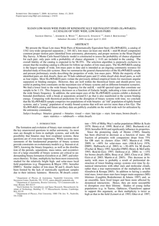
3. SLoWPoKES 3
benchmarking stellar evolutionary tracks (e.g. White et al. were not duplicate detections of the same source (PRIMARY)5 .
1999; Stassun, Mathieu, & Valenti 2007; Stassun et al. This yielded a sample of > 109 million low-mass stars with
2008), investigating the age-activity relations of M dwarfs r ∼ 14–24, at distances of ∼0.01–5 kpc from the Sun. Fig-
(e.g. Silvestri, Hawley, & Oswalt 2005), defining the ure 1 shows a graphical flow chart of the selection process and
dwarf-subdwarf boundary for spectral classification (e.g. criteria used; the steps needed in identifying kinematic com-
L´ pine et al. 2007), and calibrating the metallicity indices
e panions, which are detailed in this paper, are shown in gray
(Woolf & Wallerstein 2005; Bonfils et al. 2005). Moreover, boxes. The white boxes show subsets where kinematic infor-
equal-mass multiples can be selected to provide identical mation is not available; however, it is still possible to identify
twins with the same initial conditions (same mass, age, binary companions based on their close proximity. We will
and metallicity) to explore the intrinsic variations of stellar discuss the selection of binaries, without available kinematic
properties. In addition, wide binaries (a > 100 AU) are information, in a future paper.
expected to evolve independently of each other; even their
disks are unaffected by the distant companion (Clarke 1992). 2.2. Proper Motions
Components of such systems are effectively two single stars The SDSS/USNO-B matched catalog (Munn et al. 2004),
that share their formation and evolutionary history. In essence which is integrated into the SDSS database in the P ROPER -
they can be looked at as coeval laboratories that can be used M OTIONS table, was used to obtain proper motions for this
to effectively test and calibrate relations measured for field study. We used the proper motions from the DR7 catalog;
stars. Finally, as interest has grown in detecting exoplanets the earlier data releases had a systematic error in the calcu-
and in characterizing the variety of stellar environments in lation of proper motion in right ascension (see Munn et al.
which they form and evolve, a large sample of bona fide wide 2008, for details). This catalog uses SDSS galaxies to recali-
binaries could provide a rich exoplanet hunting ground for brate the USNO-B positions and USNO-B stellar astrometry
future missions such as SIM. as an additional epoch for improved proper motion measure-
In this paper, we present a new catalog of CPM doubles ments. The P ROPER M OTIONS catalog is resolution limited
from SDSS, each with at least one low-mass component, iden- in the USNO-B observations to 7 and is 90% complete to
tified by matching proper motions and photometric distances. g = 19.76 , corresponding to the faintness limit of the POSS-
In § 2 we describe the origin of the input sample of low-mass II plates used in USNO-B. The completeness also drops with
stars; § 3 details the binary selection algorithm and the con- increasing proper motion; for the range of proper motions in
struction of a Galactic model built to assess the fidelity of each our sample (µ = 40–350 mas yr−1 ; see § 2.3 below), the com-
binary in our sample. The resulting catalog and its character- pleteness is ∼ 85%. The typical 1 σ error is 2.5–5 mas yr−1
istics are discussed in § 4. We compare the result of our CPM for each component
double search with previous studies in § 5 and summarize our
conclusions in § 6. 2.3. Quality Cuts
2. SDSS DATA To ensure that the resultant sample of binaries is not con-
2.1. SDSS Sample of Low-Mass Stars
taminated due to bad or suspect data, we made a series of cuts
on the stellar photometry and proper motions. With > 109
SDSS is a comprehensive imaging and spectroscopic sur- million low-mass stars, we could afford to be very conserva-
vey of the northern sky using five broad optical bands (ugriz) tive in our quality cuts and still have a reasonable number of
˚
between ∼3000–10000A using a dedicated 2.5 m telescope stars in our input sample. We restricted our sample, as shown
(York et al. 2000; Fukugita et al. 1996; Gunn et al. 1998). in Figure 1, to stars brighter than r = 20 and made a cut on
Data Release Seven (DR7; Abazajian et al. 2009) contains the standard quality flags on the riz magnitudes (PEAKCEN -
photometry of 357 million unique objects over 11663 deg2 TER , NOTCHECKED , PSF FLUX INTERP, INTERP CENTER ,
of the sky and spectra of over 1.6 million objects over 9380 BAD COUNTS ERROR , SATURATED – all of which are re-
deg2 of the sky. The photometry has calibration errors of quired to be 0)7 , which are the only bands pertinent to low-
2% in u and ∼1% in griz, with completeness limits of 95% mass stars and the only bands used in our analysis.
down to magnitudes 22.0, 22.2, 22.2, 21.3, 20.5 and satura- On the proper motions, Munn et al. (2004) recommended a
tion at magnitudes 12.0, 14.1, 14.1, 13.8, 12.3, respectively minimum total proper motion of 20 mas yr−1 and cuts based
(Gunn et al. 1998). We restricted our sample to r ≤ 20 where on different flags for a “clean” and reliable sample of stellar
the SDSS/USNO-B proper motions are more reliable (see sources. Therefore, we required that each star (i) matched an
§ 2.3); hence, photometric quality and completeness should unique USNO-B source within 1 (MATCH > 0), (ii) had no
be excellent for our sample. other SDSS source brighter than g = 22 within 7 (DIST 22
Stellar sources with angular separations 0.5–0.7 are re- > 7), (iii) was detected on at least 4 of the 5 USNO-B plates
solved in SDSS photometry; we determined this empirically and in SDSS (N F IT = 6 or (N F IT = 5 and (O < 2 or J < 2))),
from a search in the N EIGHBORS table. For sources brighter (iv) had a good least-squares fit to its proper motion (SIG RA
than r ∼ 20, the astrometric accuracy is 45 mas rms per coor- < 1000 and SIG D EC < 1000), and (v) had 1 σ error for both
dinate while the relative astrometry between filters is accurate components less than 10 mas yr−1 .
to 25–35 mas rms (Pier et al. 2003). A challenge inherent in using a deep survey like SDSS
The SDSS DR7 photometric database has more than 180 to identify CPM binaries, is that most of the stars are far
million stellar sources (Abazajian et al. 2009); to select a sam- away and, therefore, have small proper motions. To avoid
ple of low-mass stars, we followed the procedures outlined in 5 We note that binaries separated by less than ∼1 might appear elongated
B10 and required r − i ≥ 0.3 and i − z ≥ 0.2, which repre- in SDSS photometry and might not be listed in the STAR table.
sents the locus of sample K5 or later dwarfs. The STAR table 6 This corresponds to r = 18.75 for K5 and r = 18.13 for M6 dwarfs.
was used to ensure that all of the selected objects had mor- 7 A PRIMARY object is already selected to not be BRIGHT and NODE -
phology consistent with being point sources (TYPE = 6) and BLEND or DEBLEND NOPEAK

4. 4 Dhital et al.
SDSS DR7 STAR
N ∼ 180 × 106
Low-mass stars
(r −i > 0.3, i−z > 0.2)
N ∼ 109 × 106
r ≤ 20 r > 20
N ∼ 28.4 × 106 N ∼ 80.6 × 106
riz & µ good
N ∼ 15.7 × 106
µ ≥ 40 mas yr−1
Input sample
N = 577459
search for companions search for companions
r ≤ 20 r > 20
∆θ ≥ 180′′ 7′′ ≤ ∆θ ≤ 180′′ ∆θ ≤ 7′′ (no µ) ∆θ ≤ 15′′ (no µ)
Match ∆µα , ∆µδ , ∆d
Match ∆d
N = 3774
riz, µ good
N = 1598
Galactic Model
Galactic Model
Pf ≤ 0.05
SLoWPoKES
N
N = 1342
Figure 1. A graphical representation of the selection process used in the identification of SLoWPoKES pairs. The gray boxes show the steps involved in
SLoWPoKES, with the results presented in this paper. The pairs without proper motions (shown in white boxes) will be presented in a follow-up paper.
confusing real binaries with chance alignments of stars at of µ = 40 mas yr−1 for our low-mass stellar sample since the
large distances, where proper motions are similar but small, number of matched pairs clearly declines with increasing ∆θ
a minimum proper motion cut needs to be applied. Figure 2 with this cutoff (Figure 2). While this still allows for a number
shows the distribution of candidate binaries (selected as de- of (most likely) chance alignments, they do not dominate the
tailed in § 3.1) with minimum proper motion cuts of 20, 30, sample and can be sifted more effectively as discussed below.
40, and 50 mas yr−1 ; the histograms have been normalized Thus, on the ∼15.7 million low-mass stars that satisfied the
by the area of the histogram with the largest area to allow for quality cuts, we further imposed a µ ≥ 40 mas yr−1 cut on
relative comparisons. All four distributions have a peak at the total proper motion that limits the input sample to 577459
small separations of mostly real binaries, but the proportion stars with excellent photometry and proper motions. As Fig-
of chance alignments at wider separations becomes larger and ure 1 shows, this input sample constitutes all the stars around
more dominant at smaller µ cutoffs. which we searched for companions. Figure 3 shows the dis-
If our aim were to identify a complete a sample of binaries, tributions of photometric distances, total proper motions, r −i
we might have chosen a low µ cutoff and accepted a relatively vs. i−z color-color diagram, and the r vs. r −z Hess diagram
high contamination of false pairs. Such was the approach in for the input sample. As seen from their r − z colors in the
the recent study of SDSS binaries by SIJ08 who used µ ≥ 15 Hess diagram, the sample consists of K5–L0 dwarfs. Metal-
mas yr−1 . Our aim, in this paper, was to produce a “pure” poor halo subdwarfs are also clearly segregated from the disk
sample with a high yield of bona fide binaries. Thus, in our dwarf population; however, due to a combination of the mag-
search for CPM pairs we adopted a minimum proper motion nitude and color limits that were used, they are also mostly K

5. SLoWPoKES 5
calibrated for solar-type stars (Ivezi´ et al. 2008) do exist
c
and can provide approximate distances for low-mass SDs,
we refrained from using them due to the large uncertainties
10-2 involved.
White dwarfs (WD): We calculated the photometric
N / Ntot
distances to WDs using the algorithm used by Harris et al.
(2006): ugriz magnitudes and the u−g, g −r, r −i, and i−z
10-3 colors, corrected for extinction, were fitted to the WD cooling
models of Bergeron, Wesemael, & Beauchamp (1995) to get
the bolometric luminosities and, hence, the distances8 . The
bolometric luminosity of WDs are a function of gravity as
10-4 well as the composition of its atmosphere (hydrogen/helium),
neither of which can be determined from the photometry.
10 20 30 40 50 60 Therefore, we assumed pure hydrogen atmospheres with
∆θ (") log g = 8.0 to calculate the distances to the WDs. As a
result, distances derived for WDs with unusually low mass
Figure 2. The angular separation distribution of candidate pairs with mini-
mum proper motions cut-offs of 20 (dotted), 30 (dashed), 40 (solid), and 50 and gravity (∼10% of all WDs) or with unusually high mass
(long dashes) mas yr−1 . These candidates were selected by matching angular and gravity (∼15% of all WDs) will have larger uncertainties.
separations, proper motions, and photometric distances as described in § 3.1. Helium WDs redder than g −i > 0.3 will also have discrepant
All histograms have been normalized by the area of the histogram with the distances (Harris et al. 2006).
largest area to allow for relative comparisons. It can be clearly deduced that a
low proper motion cut-off will cause a large proportion of chance alignments. 2.4.2. Spectral Type & Mass
We adopted a cut-off of µ ≥ 40 mas yr−1 as it allows for identification of
CPM pairs with a reasonable number of false positives that are later sifted The spectral type of all (O5–M9; −0.6 ≤ r − z ≤4.5) disk
with our Galactic model. dwarfs and subdwarfs were inferred from their r − z colors
subdwarfs and are limited to only the earliest spectral types using the following two-part fourth-order polynomial:
we probe.  2
 50.4 + 9.04 (r − z) − 2.97 (r − z) +

2.4. Derived properties 0.516 (r − z)3 − 0.028 (r − z)4 ; for O5–K5
SpT = (2)
2.4.1. Photometric Distances  33.6 + 47.8 (r − z) − 20.1 (r − z)2 −
 3 4
33.7 (r − z) − 58.2 (r − z) ; for K5–M9
Disk dwarfs (DD): We determined the distances to the DDs in
our sample by using photometric parallax relations, measured where SpT ranges from 0–67 (O0=0 and M9=67 with all
empirically with the SDSS stars. For M and L dwarfs (∼M0– spectral types, except K for which K6, K8, and K9 are not de-
L0; 0.94 < r − z < 4.34), we used the relation derived by B10 fined, having 10 subtypes) and is based on the data reported in
based on data from D. Golimowski et al. (2010, in prep.). For Covey et al. (2007) and West et al. (2008). The spectral types
higher mass dwarfs (∼O5–K9; −0.72 < r − z < 0.94), we fit should be correct to ±1 subtype.
a third-order polynomial to the data reported in Covey et al. Similarly, the mass of B8–M9 disk dwarfs and subdwarfs
(2007): were determined from their r − z colors using a two-part
fourth-order polynomial,:
Mr = 3.14+7.54 (r−z)−3.23 (r−z)2 +0.58 (r−z)3 . (1)  2
In both of the above relations, we used extinction-corrected  1.21 − 1.12 (r − z) + 1.06 (r − z) −
 3 4
2.73 (r − z) + 2.97 (r − z) ; for B8–K5
magnitudes. Ideally, Mr would have been a function of M( M ) = (3)
both color and metallicity; but the effect of metallicity is not  0.640 + 0.362 (r − z) − 0.539 (r − z)2 +
 3 4
quantitatively known for low-mass stars. This effect, along 0.170 (r − z) − 0.016 (r − z) ; for K5–M9
with unresolved binaries and the intrinsic width of the MS, based on the data reported in Kraus & Hillenbrand (2007),
cause a non-Gaussian scatter of ∼ 0.3–0.4 magnitudes in the who used theoretical models, supplemented with observa-
photometric parallax relations (West, Walkowicz, & Hawley tional constrains when needed, to get mass as a function of
2005; SIJ08; B10). Since we are matching the photometric spectral type. The scatter of the fit, as defined by the median
distances, using the smaller error bars ensures fewer false absolute deviation, is ∼2%.
matches. Hence, we adopted 0.3 magnitudes as our error, As the polynomials for both the spectral type and mass are
implying a 1 σ error of ∼14% in the calculated photometric monotonic functions of r − z over the entire range, the com-
distances. ponent with the bluer r − z color was classified as the primary
star of each binary found.
Subdwarfs (SD): Reliable photometric distance relations are
not available for SDs, so instead we used the relations for 3. METHOD
DDs above. As a result of appearing under-luminous at a 3.1. Binary Selection
given color, their absolute distances will be overestimated.
However, the relative distance between two stars in a physical Components of a gravitationally bound system are expected
binary should have a small uncertainty. Because we are to occupy the same spatial volume, described by their semi-
interested in determining if two candidate stars occupy the axes, and to move with a common space velocity. To identify
same volume in space, the relative distances will suffice. 8 SDSS ugriz magnitudes and colors for the WD
While photometric parallax relations based on a few stars cooling models are available on P. Bergeron’s website:
of a range of metallicities (Reid 1998; Reid et al. 2001b) or http://www.astro.umontreal.ca/˜bergeron/CoolingModels/

6. 6 Dhital et al.
105 105
104 104
N
N
103 103
102 102
0 1 2 3 4 100 200 300 400
distance (kpc) µ (mas yr-1)
3.0 12
2.5 14
2.0
r-i
16
r
1.5
1.0 18
0.5 20
0.5 1.0 1.5 2.0 0.5 1.0 1.5 2.0 2.5 3.0 3.5
i-z r-z
Figure 3. The characteristics of the sample of 577459 low-mass stars in the SDSS DR7 photometric catalog that forms our input sample (clockwise from top
left): the photometric distances, the total proper motions, r vs. r − z Hess diagram, and the r − i vs. i − z color–color plot. In addition to quality cuts on
proper motion and photometry, we require that stars in this sample to be low-mass (r − i ≥ 0.3 and i − z ≥ 0.2) and have a relatively high proper motion (µ ≥
40 mas yr−1 ). The contours show densities of 10–3000 in the color–color plot and 10–300 in the Hess diagram.
physical binaries in our low-mass sample, we implemented a For all pairs that were found with angular separations of
statistical matching of positional astrometry (right ascension, 7 ≤ ∆θ ≤ 180 , we required the photometric distances to
α, and declination, δ), proper motion components (µα and be within
µδ ), and photometric distances (d). The matching of distances ∆d ≤ (1 σ∆d , 100 pc) (5)
is an improvement to the methods of previous searches for
CPM doubles (L´ pine & Bongiorno 2007; Chanam´ & Gould
e e and the proper motions to be within
2004; Halbwachs 1986) and serves to provide further confi- 2 2
dence in the binarity of identified systems. ∆µα ∆µδ
The angular separation, ∆θ, between two nearby point + ≤2 (6)
σ∆µα σ∆µδ
sources, A and B, on the sky can be calculated using the small
angle approximation: where ∆d, ∆µα , and ∆µδ are the scalar differences between
the two components with their uncertainties calculated by
∆θ (αA − αB )2 cos δA cos δB + (δA − δB )2 . (4) adding the individual uncertainties in quadrature. An absolute
upper limit on ∆d of 100 pc was imposed to avoid ∆d being
We searched around each star in the input sample for all stel- arbitrarily large at the very large distances probed by SDSS;
lar neighbors, brighter than r = 20 and with good photom- hence, at d 720 pc, distances are matched to be within
etry and proper motions, within ∆θ ≤ 180 in the SDSS 100 pc and results in a significantly lower number of candi-
photometric database using the Catalog Archive Server query date pairs. The proper motions are matched in 2-dimensional
tool9 . Although CPM binaries have been found at much larger vector space, instead of just matching the total (scalar) proper
angular separations (up to 900 in Chanam´ & Gould 2004;
e motion as has been frequently done in the past. The latter
1500 in L´ pine & Bongiorno 2007; 570 in Faherty et al.
e approach allows for a significant number of false positives as
2010), the contamination rate of chance alignments at such stars with proper motions with the same magnitude but differ-
large angular separations was unacceptably high in the deep ent directions can be misidentified as CPM pairs.
SDSS imaging (see Figure 2). In addition, searching the large For our sample, the uncertainties in proper motions are
number of matches at larger separations required large com- almost always larger than the largest possible Keplerian or-
putational resources. However, since the SDSS low-mass star bital motions of the identified pairs. For example, a binary
sample spans considerably larger distances than in previous with a separation of 5000 AU and Mtot = 1 M at 200
studies (see below), our cutoff of 180 angular separation pc, which is a typical pair in the resultant SLoWPoKES sam-
probes similar physical separations of up to ∼0.5 pc, which ple, will has a maximum orbital motion of ∼0.27 mas yr−1 ,
is comparable to the typical size of prestellar cores (0.35 much smaller than error in our proper motions (typically 2.5–
pc; Benson & Myers 1989; Clemens, Yun, & Heyer 1991; 5 mas yr−1 ). However, a pair with a separation of 500 AU
Jessop & Ward-Thompson 2000). pair and Mtot = 1 M at 50 pc has a maximum orbital mo-
tion of ∼5.62 mas yr−1 , comparable to the largest errors in
9 http://casjobs.sdss.org/CasJobs/ component proper motions. Hence, our algorithm will reject

7. SLoWPoKES 7
0 120 240 360
To quantitatively assess the fidelity of each binary in our
sample, we created a Monte Carlo based Galactic model that
100 mimics the spatial and kinematic stellar distributions of the
50 N Milky Way and calculates the likelihood that a given binary
50 100 could arise by chance from a random alignment of stars.
90 90
Clearly, for this to work the underlying distribution needs to
be carefully constructed such that, as an ensemble, it reflects
60
Dec (deg)
60
the statistical properties of the true distribution. The model
needs to take into account the changes in the Galactic stellar
30 30 density and space velocity over the large range of galacto-
centric distances and heights above/below the Galactic disk
0 0 plane probed by our sample. Previous studies, focused on
nearby binaries, have been able to treat the underlying Galac-
tic stellar distribution as a simple random distribution in two-
0 120 240 360 dimensional space. For example, L´ pine & Bongiorno (2007)
e
RA (deg) assigned a random shift of 1–5◦ in Right Ascension for the
secondary of their candidate pairs and compared the resultant
Figure 4. The spatial distribution of SLoWPoKES binaries, shown in equa- distribution with the real one. As they noted, the shift cannot
torial coordinates, closely follows the SDSS footprint. The upper and right
panels show the histogram of Right Ascension and Declination in 5◦ bins. be arbitrarily large and needs to be within regions of the sky
We rejected the 118 CPM candidates found in the direction of open clus- with similar densities and proper motion systematics. With
ter IC 5146 (shown in red pluses and dashed histograms) due to the highly stars at much larger heliocentric distances in our sample, even
anomalous concentration of pairs and possibly contaminated photometry due a 1◦ shift would correspond to a large shift in Galactic position
to nebulosity (see § 3.1).
(1◦ in the sky at 1000 pc represents ∼17.5 pc). Therefore, we
such nearby, relatively tight binaries. could not use a similar approach to assess the false positives
From the mass estimates and the angular separations from in our catalog.
the resulting sample, we calculated the maximum Keplerian The Galactic model is built on the canonical view that the
orbital velocities, which are typically less than 1 mas yr−1 ; Galaxy comprises three distinct components—the thin disk,
only 104, 34, and 3 out of a total of 1342 systems exceeded the thick disk, and the halo—that can be cleanly segregated
1, 2, and 5 mas yr−1 , respectively. More importantly, only by their age, metallicity, and kinematics (Bahcall & Soneira
7 pairs had maximum orbital velocities greater than 1-σ error 1980; Gilmore, Wyse, & Kuijken 1989; Majewski 1993). We
in the proper motion; so apart from the nearest and/or tightest note that some recent work has argued for the disk to be a
pairs, our search should not have been affected by our restric- continuum instead of two distinct components (Ivezi´ et al.
c
tions on the proper motion matching in Eq. (6). 2008) or for the halo to be composed of two distinct com-
Applying these selection criteria to the stellar sample de- ponents (Carollo et al. 2008, 2009). However, for our pur-
scribed in § 2.1, we found a total of 3774 wide CPM binary poses, the canonical three-component model was sufficient.
candidates, where each has at least one low-mass component. We also did not try to model the over-densities or under-
Among these, we found 118 pairs shown in red pluses and densities, in positional or kinematic space, caused by co-
dashed histograms in Figure 4, concentrated in a 20 × 150 moving groups, open clusters, star-forming regions, or Galac-
stripe, in the direction of open cluster IC 5146.As there is sig- tic streams. If such substructures were found in the SDSS
nificant nebulosity that is not reflected in the extinction values, data, they were removed from our sample (see § 3.1). In
the photometry and, hence, the calculated photometric dis- essence, this model strictly describes stars in the field and
tances are not reliable. In addition, while the kinematics are produces the three-dimensional position and two-dimensional
not characteristic of IC 5146, they are more likely to be part proper motion, analogous to what is available for the SDSS
of a moving group rather than individual CPM pairs. Thus, photometric catalog.
we rejected all of these candidates. No other distinct struc- 3.2.1. Galactic stellar density profile
tures, in space and kinematics, were found. Then, we made
the quality cuts described in § 2.3 on the companions; 906 In the canonical Galactic model, the stellar densities (ρ) of
and 1085 companions did not meet our threshold for the pho- the thin and the thick disks, in standard Galactic coordinates
tometry and proper motions, respectively, and were rejected. R (Galactic radius) and Z (Galactic height), are given by
The majority of these rejections were near the Galactic Plane, |Z| |R−R |
−H −
which was expected due to higher stellar density. Thus, at the ρthin (R, Z) = ρ (R , 0) e thin e Lthin
(7)
end, the resulting sample had 1598 CPM double candidates −H
|Z| |R−R |
− L
from the statistical matching (Figure 1). Inherent in statistical ρthick (R, Z) = ρ (R , 0) e thick e thick , (8)
samples are false positives, arising from chance alignments where H and L represent the scale height above (and below)
within the uncertainties of the selection criteria. For any star, the plane and the scale length within the plane, respectively.
the probability of chance alignment grows with the separation The halo is described by a bi-axial power-law ellipsoid
making the wider companions much more likely to be chance
rhalo
alignments despite the selection criteria we just implemented. R
Hence, it is necessary to complete a detailed analysis of the ρhalo (R, Z) = ρ (R , 0) (9)
fidelity of the sample. R2 + (Z/q)2
3.2. Galactic Model: Assessing False Positives in the Binary
with a halo flattening parameter q and a halo density gradient
Sample rhalo . The three profiles are added together, with the appro-
priate scaling factors, f , to give the stellar density profile of

8. 8 Dhital et al.
Table 1 Table 2
Galactic Structure Parameters Galactic Kinematics
Component Parameter name Parameter description Adopted Value Galactic component Velocity k n
ρ (R , 0) stellar density 0.0064 U 7.09 0.28
fthin fractiona 1-fthick -fhalo thin disk V 3.20 0.35
thin disk Hthin scale height 260 pc W 3.70 0.31
Lthin scale length 2500 pc U 10.38 0.29
fthick fractiona 9% thick disk V 1.11 0.63
thick disk Hthick scale height 900 pc W 0.31 0.31
Lthick scale length 3500 pc
fhalo fractiona 0.25%
Note. — The constants in the power law,
halo rhalo density gradient 2.77
σ(Z) = k|Z|n , that describes the velocity
q (= c/a)b flattening parameter 0.64 dispersions of the stars in the thin and thick
disks. The velocity dispersions were measured
Note. — The parameters were measured using M dwarfs for the from a spectroscopic sample of low-mass dwarfs
disk (Bochanski et al. 2010) and main-sequence turn-off stars for the halo (Bochanski et al. 2007).
(Juri´ et al. 2008) in the SDSS footprint.
c
a Evaluated in the solar neighborhood coordinates, as:
b Assuming a bi-axial ellipsoid with axes a and c
Vr (Z) = 0
the Galaxy: Vφ (Z) = Vcirc − Va − f (Z) (11)
ρ (R, Z) = fthin ρthin + fthick ρthick + fhalo ρhalo . (10) Vz (Z) = 0,
The scaling factors are normalized such that fthin + fthick + where Vcirc = 220 km s−1 , Va = 10 km s−1 , f (Z) =
fhalo = 1. With the large number of stars imaged in the 0.013 |Z| − 1.56 × 10−5 |Z|2 was derived by fitting a poly-
SDSS, robust stellar density functions have been measured for nomial to the data in West et al. (2008), and Z is in par-
the thin and thick disks using the low-mass stars (Juri´ et al.
c secs. This formulation of Vφ (Z) is consistent with a stel-
2008; B10) and for the halo using the main-sequence turn-off lar population composed of a faster thin disk ( Vφ = 210
stars (Juri´ et al. 2008). The values measured for the disk in
c km s−1 ) and a slower thick disk ( Vφ = 180 km s−1 ).
the two studies are in rough agreement. We adopted the disk Then, we converted these galactocentric polar velocities to
parameters from B10 and the halo parameters from Juri´ et al.
c the heliocentric, Cartesian UVW velocities. The UVW veloc-
(2008); Table 1 summarizes the adopted values. ities, when complemented with the dispersions, can be con-
verted to a two-dimensional proper motion (and radial veloc-
ity; Johnson & Soderblom 1987), analogous to our input cat-
alog. We used the UVW velocity dispersions measured for
3.2.2. Galactic Kinematics SDSS low-mass dwarfs (Bochanski et al. 2007). All the dis-
Compared to the positions, the kinematics of the stellar persions were well described by the power-law
components are not as well characterized; in fact, apart from σ(Z) = k |Z|n , (12)
their large velocity dispersions, little is known about the halo
kinematics. We seek to compare the proper motions of a where the values of constants k and n are summarized in Ta-
candidate pair with the expected proper motions for that pair ble 2. As the velocity dispersions in Bochanski et al. (2007)
given its Galactic position. Thus, we found it prudent to (i) ig- extend only up to ∼1200 pc, we extrapolated the above equa-
nore the halo component, with its unconstrained kinematics, tion for larger distances. While the velocity ellipsoids of F
at distances where its contributions are expected to be mini- and G dwarfs have been measured to larger distances (e.g.
mal and (ii) limit our model to a distance of 2500 pc, which Bond et al. 2009), we preferred to use the values measured
corresponds to the Galactic height where the number of halo for M dwarfs for our low-mass sample.
stars begins to outnumber disk stars (Juri´ et al. 2008). In
c
practice, all the SLoWPoKES CPM pairs, with the exceptions
of subdwarfs for which distances were known to be overesti-
3.2.3. The Model
mated, were within ∼1200 pc (see Figure 9 below); so we did
not introduce any significant systematics with these restric- By definition, a chance alignment occurs because two phys-
tions. ically unassociated stars randomly happen to be close together
An ensemble of stars in the Galactic Plane can be character- in our line of sight (LOS), within the errors of our measure-
ized as having a purely circular motion with a velocity, Vcirc . ments. Due to the random nature of these chance alignments,
The orbits become more elliptic and eccentric over time due it is not sufficient to estimate the probability of chance align-
to kinematic heating causing the azimuthal velocity, Vφ , to ment along a given LOS simply by integrating Eq. (10). This
decrease with the Galactic height, Z. However, the mean ra- would tend to underestimate the true number of chance align-
dial (Vr ) and perpendicular (Vz ) velocities for the ensemble ments because the density profiles in Eqs. (7–9) are smooth
at any Z remains zero, with a given dispersion, as there is no functions that, in themselves, do not include the random scat-
net flow of stars in either direction. In addition, this random- ter about the mean relation that real stars in the real Galaxy
ization of orbits also causes the asymmetric drift, Va , which have. Thus, the stars need to be randomly redistributed spa-
increases with the age of stellar population and is equivalent tially about the average given by Eq. (10) in order to properly
to ∼10 km s−1 for M dwarfs. Hence, the velocities of stars in account for small, random fluctuations in position and veloc-
the Galactic disk can be summarized, in Galactic cylindrical ity that could give rise to false binaries in our data.

9. SLoWPoKES 9
In principle, one could simulate the whole Galaxy in this
fashion in order to determine the probabilities of chance align- 1
ments as a function of LOS. In practice, this requires exorbi-
tant amounts of computational time and memory. Since our
aim was to calculate the likelihood of a false positive along 10-1
specific LOSs, we, instead, generated stars in much smaller
<N>
regions of space, corresponding to the specific binaries in our
sample. For example, a 30 × 30 cone integrated out to a 10-2
distance of 2500 pc from the Sun will contain at least a few
thousand stars within any of the specific LOSs in our sample.
The number of stars is large enough to allow for density vari- 10-3
ations similar to that of the Milky Way while small enough to
be simulated with ease. With a sufficient number of Monte
Carlo realizations, the random density fluctuations along each
LOS can be simulated. We found that 105 realizations allowed 10 100
for the results to converge, within ∼0.5%. ∆θ (")
We implemented the following recipe to assess the false-
positive likelihood for each candidate pair using our Galactic Figure 5. The distribution of the (average) number of stars found around the
LOSs around our binary candidates as calculated from the SDSS DR7 data
model: (solid histograms) and our Galactic model (dashed histograms). All optical
pairs (red), pairs with matching distances (blue), and pairs with matching
(i) The total number of stars in the LOS volume defined distances and proper motion components (purple) are shown. The excess at
by a 30 × 30 area, centered on the α and δ of a given small separations, a signature of real pairs, is enhanced as additional proper-
ties are matched. Unlike the rest of the paper, we counted all stars with r ≤
binary, over heliocentric distances of 0–2500 pc was 22.5, without any quality cuts, for this plot to do a realistic comparison with
calculated by integrating Eq. (10) in 5 pc deep, discrete the model. Note that N denotes the number of stars found at that angular
cylindrical “cells.” separation (counted in 1 bins). We used the raw parameters for the Galactic
model (Juri´ et al. 2008, B10). As a whole, the model does an excellent job
c
Integrating Eq. (10) for ∆θ = 30 and d = 0–2500 pc of mimicking the number of stars and their spatial and kinematic distribution
resulted in ∼3300–1580 stars, with the higher numbers in the Milky Way along typical SDSS LOSs.
more likely to be the LOSs along the Galactic Plane. tions for LOSs at large distances were expected. Devi-
This number of stars, when randomly redistributed in ations for LOSs at low Galactic latitudes are reasonable
the entire volume, was more than enough to recreate as the parameters in Eqs. (7) and (8) as not as well con-
over-densities and under-densities. strained along the Galactic disk. Hence, we concluded
that the rejection method used in redistributing the stars
(ii) The stars were then distributed in three-dimensional in the 30 × 30 LOS is correctly implemented and that
space defined by the LOS using the rejection method the model successfully replicates the three dimensional
(Press et al. 1992), generating α, δ, and d for each star. spatial distribution of the stars in the Galaxy.
The rejection method ensured that the stars were ran-
domly distributed while following the overlying distri- When the distances were matched, the number of pairs
bution function, which, in this case, was the stellar den- decreased as chance alignments were rejected (blue his-
sity profile given by Eq. (10). tograms in Figure 5); there are, on average, only ∼0.41
and ∼3.6 chance alignments within 60 and 180 , re-
The model did an excellent job of replicating the ac- spectively. Note that matching distances, in addition to
tual distribution of stars in the three-dimensional space. the angular separation, significantly enhanced the peak
The red histograms in Figure 5 show the number of at the small separations.
stars from the center of the LOS as a function of an-
gular separation for the model (dashed lines) and the (iii) Based on the Galactic position of each randomly gener-
data (solid lines), averaged over all LOSs where candi- ated star, mean UVW space velocities and their disper-
date binaries were identified in § 3.1. There is an ex- sions were generated based on Eq. (11) and Eq. (12),
cess of pairs at close separations, a signature of gen- respectively. Proper motions were then calculated
uine, physically associated pairs, while the two distri- by using the inverse of the algorithm outlined in
butions follow the same functional form at larger sep- Johnson & Soderblom (1987). These generated proper
arations, where chance alignments dominate. The in- motions represent the expected kinematics of stars at
creasing number of pairs with angular separation is an the given Galactic position.
evidence of larger volume that is being searched. In- Figure 6 shows the comparison between the proper mo-
tegrating the model predicts ∼8.0 stars within a search tions in the SDSS/USNO-B catalog and our model;
radius of 60 and ∼71 within 180 . In other words, for component proper motions of stars within 60 of all
a typical LOS with candidate binaries, we would, on LOSs, where candidate pairs were found. For the pur-
average, expect to find 8 chance alignments within 60 poses of this plot, we restricted the stars to be within
and ∼71 within 180 when considering only angular 1200 pc and of spectral type K5 or later so we could
separation. compare kinematics with a sample similar to our resul-
For the 180 radius around each LOS, the average num- tant catalog. We also did not compare the distributions
ber of stars in the model and the data were within a few at µα or µδ < 10 mas yr−1 where the proper motions
σ of each other, with the largest deviations found along are comparable to the 1-σ errors and, hence, not reli-
the LOSs at low Galactic latitudes or large distances. able. Since our initial sample was has µ ≥ 40 mas yr−1 ,
As our model only integrated to d = 2500 pc, devia- stars with the small proper motion component are either

10. 10 Dhital et al.
1.0
(µα and µδ ), same as is available for SDSS photometric cata-
µα µδ log. Based on the above results, we concluded that the Galac-
0.8 tic model sufficiently reproduced the five-dimensional (three
spatial and two kinematic10 ) distribution of stars along typical
SDSS/USNO-B
model
0.6
LOSs in the Milky Way and, thus, allowed for the calculation
of probability that a given CPM double is a chance alignment.
N
0.4
0.2 3.3. Fidelity
0.0 As described in the previous section, we have implemented
-100 0 100 -100 0 100
a very stringent selection algorithm in identifying the CPM
µ (mas yr-1) pairs. In addition to only including objects with the most ro-
Figure 6. Proper motion distributions for stars within 60 of LOSs along all
bust photometry and proper motions, we also used a relatively
identified candidate pairs in SDSS/USNO-B (solid histograms) and in our high proper motion cut of µ ≥ 40 mas yr−1 for the input sam-
Galactic model (dashed histograms). For the purposes of this plot, we re- ple, which considerably decreased the number of low-mass
stricted the stars to be of spectral types K5 or later and be within 1200 pc to stars. As described above, an algorithm optimized to reject
avoid being skewed by systematic differences. In addition, we do not com-
pare proper motion components < 10 mas yr−1 as they comparable to the
the most false positives, even at the expense of real pairs, was
1-σ errors and, hence, not reliable (see text). Again, the kinematics of the used in the statistical matching of angular separation, photo-
thin and thick disk of the Milky Way are very well reproduced by our Monte metric distance, and proper motion components. Lastly, we
Carlo model. used the Galactic model to quantify the probability of chance
alignment, Pf , for each of the 1558 candidate pairs.
rejected or their motion is dominated by the other com- Normally all candidate pairs with Pf ≤ 0.5, i.e. a higher
ponent in our analysis. As evidenced in the figure, our chance of being a real rather than a fake pair, could be used
model reproduced the overall kinematic structure of the to identify the binaries. However, to minimize the number of
thin and thick disks. spurious pairs, we required
When the proper motions were matched (purple his- Pf ≤ 0.05. (13)
tograms in Figure 5), in addition to the angular sepa-
ration and distances, the number of chance alignments for a pair to be classified as real. Here we note that Pf rep-
fell drastically, especially at the smaller separations. In resents the false-alarm probability that a candidate pair iden-
fact, at ∆θ ≤ 15 , there were < 10−4 chance align- tified by matching angular separation, photometric distance,
ments, on average; even at ∆θ= 180 , the real pairs and proper motion components, as described by Eqs. (5) and
outnumbered the chance alignments by a factor of 4– (6), is a real pair; it is not the probability that a random low-
5. Cumulatively, for a typical LOS, there were, on mass star is part of a wide binary.
average, only ∼0.0097 and ∼0.086 chance alignments Making the above cut on Pf resulted in a catalog of 1342
within 60 and 180 , respectively. As a result of match- pairs, with a maximum of 5% or 67 of the pairs expected to
ing distance and proper motions components, the num- be false positives. However, as a large number of the pairs
ber of chance alignments within 180 were reduced by have extremely small Pf (see Figure 7), the number of false
a factor of ∼800. positives is likely to be much smaller. Adding up the Pf for
the pairs included in the catalog gives an estimated 22 (1.65%)
(iv) In the model galaxy, we repeated the selection process false positives. In other words, the overall fidelity of SLoW-
used to find CPM pairs in the SDSS photometric cat- PoKES is 98.35%. This is a remarkably small proportion for
alog, as described in § 3.1. To avoid double-counting, a sample of very wide pairs, especially since they span a large
the input coordinates of the LOS were considered to be range in heliocentric distances and is a testament to our selec-
the primary star. Note that we did not intend to model tion criteria. For example, if the proper motion components
and reproduce both stars of a given pair but wanted to were matched to within 2 σ, Eq. (13) would have rejected
see if a random chance alignment could produce a com- 60% of the candidates. Our choice of Eq. (13) is a matter of
panion for a given primary. Hence, each additional star preference; if a more efficient (or larger) sample is needed, it
that was found to satisfy Eqs. (5) and (6) was counted can be changed to suit the purpose.
as an optical companion. The average number of com- To get a first-order approximation of how many real bi-
panions found in the 105 Monte Carlo realizations is the naries we are missing or rejecting, we applied our selec-
probability of chance alignment or the probability that tion algorithm to the rNLTT CPM catalog with 1147 pairs
the candidate pair is a false positive, Pf , for that candi- (Chanam´ & Gould 2004). Note that Chanam´ & Gould
e e
date pair. The number of realizations sets the resolution (2004) did not match distances of the components, as they did
of Pf at 10−5 . not have reliable distance estimates available and matched to-
tal proper motions instead of a two-dimensional vector match-
(v) Finally, this was repeated for all candidate pairs that ing in our approach. Out of the 307 rNLTT pairs, which have
were found in § 3.1. Figure 7 shows the distribution ∆θ ≤ 180 and are within the SDSS footprint, we recover
of Pf all of the candidate pairs; we further discuss this both components of 194 systems (63%) and one component
distribution is § 3.3. of another 56 (18%) systems, within 2 of the rNLTT coordi-
To conclude, the result of our Galactic model was a 30 ×30 nates. Of the 194 pairs for which both components had SDSS
area of the sky, centered around the given CPM pair, with the counterparts, 59 (30%) pairs satisfied our criteria for proper
surrounding stars following the Galactic spatial and kinematic 10 The model also predicts radial velocities. We have an observational
distributions of the Milky Way. Each star in this model galaxy program underway to obtain radial velocities of the binaries for further re-
was described by its position (α, δ, and d) and proper motion finement of the sample.

11. SLoWPoKES 11
the images are from the SDSS database. In the collage high-
mass ratio pairs (top row; mass ratio = m2 /m1 < 0.5), equal-
150 mass pairs (middle row; having masses within ∼5% of each
other), white dwarf–disk dwarf pairs (bottom row, left), and
100 halo subdwarf pairs (bottom row, right) are shown. Table 4
summarizes the different types of systems in the catalog.
N
50
In the sections that follow, we summarize various aspects
of the systems that constitute the SLoWPoKES catalog and
0 briefly examine some of the follow-up science that can be
pursued with SLoWPoKES. We wish to emphasize that the
-5 -4 -3 -2 -1 0 SLoWPoKES catalog is intended principally as a high-fidelity
log Pf sample of CPM doubles that can be used for a variety of
follow-up investigations where the reliability of each object
Figure 7. The probability of chance alignment (Pf ) for candidate SLoW- in the catalog is more important than sample completeness.
PoKES pairs based on their positions and kinematics, as calculated by our Thus, we have not attempted to fully account for all sources
Galactic model. We adopted Pf = 0.05 (dotted line) as our threshold for of incompleteness or bias; and we intentionally have not ap-
inclusion in the SLoWPoKES catalog. The resolution of the Monte Carlo
simulation is 10−5 , which causes the peak at log Pf = 10−5 . plied any form of statistical “corrections” to the catalog.
motions, Eq. (6), while 19 (10%) pairs satisfied our criteria for We note that some of the most important sources of incom-
both proper motions and distances, Eqs. (5) and (6). In other pleteness in the present catalog could be at least partially over-
words with our selection criteria, we recovered only 10% of come with follow-up observations. For example, the prin-
the rNLTT pairs, with SDSS counterparts, as real binaries. If cipal incompleteness in SLoWPoKES arises from the lack
we relax our selection criteria to match within 2-σ, the num- of proper motions for SDSS stars that were not detected in
ber of recovered pairs increases to 82 with matching proper USNO-B. Proper motions either do not exist or are not reliable
motions and 37 with matching proper motions and distances. for stars (i) fainter than r = 20 or (ii) within 7 of a brighter
Of course, as the rNLTT is a nearby, high proper motion cat- star. The first criterion currently rules out most of the mid–
alog, Chanam´ & Gould (2004) had to allow for larger differ-
e late M dwarf companions, while the latter rejects close bina-
ences in proper motions due to the stars’ orbital motion, which ries and most hierarchical higher-order systems. However, as
is not applicable to the SLoWPoKES sample (see § 3.1). In the SDSS photometric and astrometric data are available for
conclusion, compared to previous catalogs of CPM doubles, these systems, their multiplicity could be verified with more
we find a small fraction of previously identified very wide bi- rigorous analysis or through cross-matching with other cata-
naries. The reasons for the low recovery rate are two-fold: logs. For example, by cross-matching SDSS with 2MASS,
(i) the restrictive nature of our matching algorithm that rejects an M4.5–L5 binary (Radigan et al. 2008) and an M6–M7 bi-
the most false positives, even at the expense of real pairs and nary (Radigan et al. 2009) have already been identified. At
(ii) improvement in the identification method—e.g. matching the other end of the spectrum, SDSS saturates at r ≈ 14, re-
proper motions in vector space and being able to use photo- sulting in saturated or unreliable photometry for the brighter
metric distance as an additional criterion. stars. We found that more than 1000 candidate pairs were
rejected for this reason; with reliable follow-up photometry
these could be added as additional genuine SLoWPoKES bi-
naries.
Even so, a fully volume-complete sample is likely to be im-
possible to compile over the full ranges of spectral types and
4. CHARACTERISTICS OF THE SLoWPoKES CATALOG distances spanned by our catalog. For example, our magni-
Using statistical matching of angular separation, photomet- tude limits of 14 r ≤ 20 imply that while we are sensi-
ric distance, and proper motion components, we have iden- tive to K5 dwarfs at ∼250–3900 pc, we are sensitive to M5
tified 1598 very wide, CPM double candidates from SDSS dwarfs at ∼14–180 pc. This means (i) we are entirely insen-
DR7. We have built a Galactic model, based on empirical sitive to pairs with the most extreme mass ratios (i.e. a K5
measurements of the stellar density profile and kinematics, to paired with an M6 or M7) and (ii) we cannot directly com-
quantitatively evaluate the probability that each of those can- pare the properties of K5 and M5 spectral subtypes in iden-
didate doubles are real (Figure 7). Using Eq. (13), we clas- tical distance ranges. In addition, as illustrated in Figure 9,
sify 1342 pairs as real, associated pairs. In deference to their with our 7 ≤ ∆θ ≤ 180 search radius we are sensitive to
extremely slow movement around each other, we dub the re- companions with separations of ∼700–18000 AU at 100 pc
sulting catalog SLoWPoKES for Sloan Low-mass Wide Pairs but ∼7000–180000 AU at 1000 pc. Thus, it is important with
of Kinematically Equivalent Stars. Table 4 lists the properties the current catalog that statistical determinations of ensem-
of the identified pairs. The full catalog is publicly available ble system properties be performed within narrowly defined
on the world wide web11 . SLoWPoKES is intended to be a slices of separation and distance. We do so in the follow-
“live” catalog of wide, low-mass pairs, i.e., it will be updated ing subsections as appropriate; but we emphasize again that
as more pairs are identified and as follow-up photometric and our intent here is primarily to characterize the SLoWPoKES
spectroscopic data become available. sample and will proffer any interpretive conclusions only ten-
Figure 8 shows a collage of gri composite images, 50 on tatively.
a side, of a selection of representative SLoWPoKES systems; Finally, as is evident from Table 4, the current SLoW-
PoKES catalog is clearly not well suited for study of higher-
11 http://www.vanderbilt.edu/astro/slowpokes/ order multiples (i.e. triples, quadruples, etc.). Identifying

12. 12 Dhital et al.
Table 3
Properties of SLoWPoKES pairs
IDa Position (J2000) Photometryb
αA δA αB δB rA iA zA rB iB zB
SLW (deg) (mag)
J0002+29 0.515839 29.475183 0.514769 29.470617 16.79 (0.02) 15.85 (0.02) 15.33 (0.02) 19.35 (0.02) 17.91 (0.02) 17.17 (0.02)
J0004-10 1.122441 -10.324043 1.095927 -10.296753 18.25 (0.02) 17.08 (0.02) 16.46 (0.02) 18.66 (0.02) 17.42 (0.02) 16.70 (0.02)
J0004-05 1.223125 -5.266612 1.249632 -5.237299 14.85 (0.01) 14.31 (0.01) 14.02 (0.02) 19.56 (0.02) 18.10 (0.01) 17.31 (0.02)
J0005-07 1.442631 -7.569930 1.398478 -7.569359 17.35 (0.02) 16.25 (0.01) 15.65 (0.01) 18.78 (0.02) 17.43 (0.02) 16.69 (0.01)
J0005+27 1.464802 27.325805 1.422484 27.300282 18.91 (0.02) 17.63 (0.02) 16.94 (0.01) 19.79 (0.02) 18.29 (0.02) 17.50 (0.02)
J0006-03 1.640868 -3.928988 1.641011 -3.926589 17.06 (0.01) 16.01 (0.02) 15.44 (0.01) 17.88 (0.01) 16.62 (0.02) 15.93 (0.01)
J0006+08 1.670973 8.454040 1.690136 8.498541 19.48 (0.02) 18.14 (0.02) 17.45 (0.02) 19.57 (0.02) 18.15 (0.01) 17.43 (0.02)
J0007-10 1.917002 -10.340915 1.924510 -10.338869 17.43 (0.01) 16.50 (0.01) 16.02 (0.03) 18.33 (0.01) 17.24 (0.01) 16.66 (0.03)
J0008-07 2.135590 -7.992694 2.133660 -7.995245 17.33 (0.01) 16.35 (0.02) 15.86 (0.02) 18.14 (0.01) 16.98 (0.02) 16.36 (0.02)
J0009+15 2.268841 15.069630 2.272453 15.066457 18.52 (0.02) 17.00 (0.02) 16.09 (0.01) 18.39 (0.02) 16.83 (0.02) 15.95 (0.01)
Table 3
Proper Motion Distancec Spectral Typed Binary Information
µαA µδA µαB µδB dA dB A B ∆θ ∆µ ∆d BE Pf Classe
( mas yr−1 ) (pc) ( ) ( mas yr−1 ) (pc) (1040 ergs) (%)
198 (2) 38 (2) 197 (3) 35 (3) 341 301 M1.7 M3.6 16.8 2.9 39 58.08 0.000 SD
43 (3) -4 (3) 36 (4) -8 (4) 362 338 M2.7 M3.1 135.9 7.5 23 3.94 0.036 DD
101 (2) 11 (2) 99 (4) 8 (4) 301 333 K7.1 M3.8 142.0 3.1 31 13.45 0.006 DD
30 (2) -21 (2) 30 (3) -27 (3) 296 273 M2.4 M3.4 157.6 6.0 23 4.90 0.015 DD
10 (3) -40 (3) 5 (4) -40 (4) 357 380 M3.1 M3.9 163.6 5.5 22 2.26 0.037 DD
-40 (2) -35 (2) -40 (2) -31 (2) 242 270 M2.2 M3.1 8.7 3.9 27 112.47 0.005 DD
-48 (4) -5 (4) -41 (4) -3 (4) 417 476 M3.3 M3.5 174.1 7.5 58 1.59 0.033 DD
37 (3) 34 (3) 42 (4) 31 (4) 429 445 M1.5 M2.3 27.6 5.6 16 27.74 0.034 DD
-9 (2) -42 (2) -7 (3) -41 (3) 344 379 M1.7 M2.7 11.5 2.3 34 74.69 0.017 DD
36 (3) -16 (3) 37 (3) -21 (3) 150 161 M4.2 M4.2 17.0 4.8 11 21.02 0.004 DD
Note. — The first 10 pairs are listed here; the full version of the table is available online.
a The identifiers were generated using the standard Jhhmm±dd format using coordinates of the primary star and are prefaced with the string ’SLW’.
b All magnitudes are psfmag and have not been corrected for extinction. Their errors are listed in parenthesis. Note that we use extinction-corrected
magnitudes in our analysis.
c The distances were calculated using photometric parallax relations and have 1 σ errors of ∼14%. The absolute distances to subdwarfs (SDs) are
overestimated (see §2.4.1).
d The spectral types were inferred from the r − z colors (West et al. 2008; Covey et al. 2007) and are correct to ±1 subtype.
e Class denotes the various types of pairs in SLoWPoKES. See Table 4.
CPM triples are identified in our search (Table 4). Moreover,
Table 4 the current SLoWPoKES catalog is likely to contain quadru-
The SLoWPoKES binaries
ple systems in which the two components of the identified
Class Type Number wide binary are themselves in fact spatially unresolved bina-
ries with near-equal mass components. We have initiated an
DD disk dwarf 1245
SD subdwarf 70
adaptive optics program to identify such higher-order systems
WD white dwarf–disk dwarf 21 in the SLoWPoKES catalog.
T triple 4
4.1. Kinematic Populations
Luyten (1922) devised the reduced proper motion (RPM)
CPM higher-order multiple systems in SDSS is very chal- diagram to be used in the stead of the H-R diagram when dis-
lenging due to the lack of reliable proper motions in the tances to the objects are not available, as is the case in large
SDSS/USNO-B matched catalog at ∆θ < 7 and r > 20. imaging surveys. The RPM of an object is defined as
Unless all components are widely separated and are all bright, H ≡ m + 5 log µ + 5 = M + 5 log vt − 3.25 (14)
they will be rejected in our search. In addition, we are cur-
rently rejecting hierarchical triples consisting of a close pair where vt is the heliocentric tangential velocity in km s−1
that is unresolved in SDSS and a wide, CPM tertiary. If the given by vt = 4.74 µ d and µ is the proper motion in arcsec-
mass ratio of the close, unresolved pair is near unity, it will onds yr−1 . Just as in a H-R diagram, the RPM diagram effec-
appear as an over-luminous single star that will then be mis- tively segregates the various luminosity or kinematic classes
interpreted by our algorithm as having a discrepant photo- from each other (e.g. Chanam´ & Gould 2004; Harris et al.
e
metric distance from its wide tertiary companion. The avail- 2006; L´ pine & Bongiorno 2007; SIJ08).
e
able SDSS photometry and astrometry shows evidence of a WDs, in addition to being relatively very blue, are less lu-
substantial number of such multiple systems, and we plan minous than either the DDs or the SDs; hence, the observed
to make these the subject of a future study. Already, four WDs tend to be nearby disk WDs with high tangential ve-