The document describes two mini-projects analyzing Twitter data: 1. It analyzes the prominence of followers for celebrities Britney Spears, Mariah Carey, and Ashley Tisdale by calculating a prominence ratio and finding statistics. It finds Mariah Carey has the most prominent followers based on the median ratio. 2. It extracts tweets from Seattle, WA and Southampton, UK containing phrases like "I want pizza" and "I want to sleep" to compare preferences. It also analyzes tweets with "Monday" vs "Friday" to study mood. It finds pizza is more popular in Seattle tweets while sleep is slightly more popular in Southampton tweets. Both cities seem more negative on Mondays than thankful

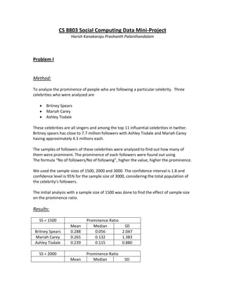
1. CS 8803 Social Computing Data Mini-Project
Harish Kanakaraju Prashanth Palanthandalam
Problem I
Method:
To analyze the prominence of people who are following a particular celebrity. Three
celebrities who were analyzed are
 Britney Spears
 Mariah Carey
 Ashley Tisdale
These celebrities are all singers and among the top 11 influential celebrities in twitter.
Britney spears has close to 7.7 million followers with Ashley Tisdale and Mariah Carey
having approximately 4.3 millions each.
The samples of followers of these celebrities were analyzed to find out how many of
them were prominent. The prominence of each followers were found out using
The formula “No of followers/No of following”, higher the value, higher the prominence.
We used the sample sizes of 1500, 2000 and 3000. The confidence interval is 1.8 and
confidence level is 95% for the sample size of 3000, considering the total population of
the celebrity’s followers.
The initial analysis with a sample size of 1500 was done to find the effect of sample size
on the prominence ratio.
Results:
SS = 1500 Prominence Ratio
Mean Median SD
Britney Spears 0.288 0.056 2.047
Mariah Carey 0.265 0.132 1.383
Ashley Tisdale 0.239 0.115 0.880
SS = 2000 Prominence Ratio
Mean Median SD

2. Britney Spears 0.546 0.111 3.067
Mariah Carey 0.289 0.163 1.230
Ashley Tisdale 0.406 0.130 7.007
SS = 3000 Prominence Ratio
Mean Median SD
Britney Spears 0.493 0.081 3.403
Mariah Carey 0.258 0.154 1.014
Ashley Tisdale 0.348 0.133 5.734
P value 0.03631 (X2 = 6.6258)
Basic Analysis:
The mean and the standard deviation may swing either ways based on the sample due
to the outliers. If the sample contains one very prominent person, it would boost the
mean and SD values. But the median trend always remains the same.
Using Median: Mariah Carey has prominent followers than Ashley Tisdale. And Ashley
Tisdale has more prominent followers than Britney spears.
From Fig 1, we can see that Britney spears has relatively high number of low prominent
followers (ratio close to zero), while Ashley and Mariah have large number of followers
with a decent prominence value, while number of followers for Britney in this region is
low. That’s why her median is the lowest among the three.
From Fig 2, we can find that Britney Spears has relatively more number of very
prominent followers compared to Ashley and Mariah. But the very prominent followers
are very very less in number compared to the whole population set.
R Commands used:
The below sequence was executed for the three celebrities,
at4 <- getUser("ashleytisdale")
at4Fl <- at4$getFollowers(n=3000)
at4FFl <- sapply(at4Fl,followersCount)
at4FFd <- sapply(at4Fl,friendsCount)
at4Ratio <- mapply("/", at4FFl, at4FFd)
med <- median(sort(at4Ratio))
stad<- sd(at4Ratio)
meanRatio <- mean(at4Ratio)
at4sum <- sum(at4Ratio)

3. Chi-square test
Chisq.test(c(at4sum,bs4sum,mc4sum))
Plotting graph (executed only once)
xyz <- cbind(bs4Ratio, at4Ratio, mc4Ratio, deparse.level = 1)
data = melt(xyz, id=c("bs4Ratio"))
lowProminence <- qplot(value, data = data, geom = "histogram", color = X2, binwidth =
50)
highP <- ggplot(data, aes(x=X2, y=value))
highP + geom_point(position = "jitter")
Fig 1: Low prominent followers
Fig 2: High prominent followers

4. Problem II
Method:
To extract tweets from two different geographic locations in the world, and select the
tweets which contain the phrase “I want”. A comparison of preferences of the twitter
users from the two locations has been done, with respect to the terms “I want a pizza”
and “I want to sleep”. Also, the mood of the users on Monday and Friday has been
studied, by extracting the tweets with the terms “Monday” and “I hate”; and “Friday”
and “Thank God”.
The searchTwitter() functionality of the twitteR package for R Studio has been used.
The two cities chosen were Seattle, Washington and Southampton, UK.

5. 1000 tweets with the phrase “I want” were extracted within a 20 mile radius of the two
cities.
southamTweets = searchTwitter("I
want",1000,NULL,NULL,NULL,NULL,'50.903,-1.40625,20mi',NULL)
The list of 1000 tweets is then converted into text form by using the lapply() command.
southamTweets.text = lapply(southamTweets, function(southampton)
southampton$getText())
The grep() command is used to extract incidences of the term “pizza” in the tweet list.
southamTweets.spec = grep("pizza",southamTweets.text,TRUE)
The procedure is repeated for Seattle:
seattleTweets = searchTwitter("I
want",1000,NULL,NULL,NULL,NULL,'47.606,-122.299,20mi',NULL)
> seattleTweets.text = lapply(seattleTweets,function(seattle)
seattle$getText())
> seattle.spec = grep("pizza",seattleTweets.text,TRUE)
Variations of the “I want a pizza” phrase have also been tried.
seattleSpecific.spec = grep("I want pizza",seattleTweets.text,TRUE)
Instead of “pizza”, the tweets containing the phrase “sleep” or “I want to sleep” were
used.
southamTweetsSleep.spec = grep("sleep",southamTweets.text,TRUE)
southamTweetsSleepSpecific.spec = grep("I want to
sleep",southamTweets.text,TRUE)
seattleSleep.spec = grep("sleep",seattleTweets.text,TRUE)
seattleSleepSpecific.spec = grep("I want to
sleep",seattleTweets.text,TRUE)
seattleSleepSpecific.spec = grep("I want
sleep",seattleTweets.text,TRUE)
Another variant of the above experiment was done, with the terms “Monday” and
“Friday” and respectively, the phrases “I hate” and “Thank God”

6. seattleMonday =
searchTwitter("Monday",1000,NULL,NULL,NULL,NULL,'47.606,-
122.299,20mi',NULL)
> seattleFriday =
searchTwitter("Friday",1000,NULL,NULL,NULL,NULL,'47.606,-
122.299,20mi',NULL)
> southamMonday = searchTwitter("I
want",1000,NULL,NULL,NULL,NULL,'50.903,-1.40625,20mi',NULL)
> southamMonday =
searchTwitter("Monday",1000,NULL,NULL,NULL,NULL,'50.903,-
1.40625,20mi',NULL)
> southamFriday =
searchTwitter("Friday",1000,NULL,NULL,NULL,NULL,'50.903,-
1.40625,20mi',NULL)
> southamMonday.text = lapply(southamMonday, function(southampton)
southampton$getText())
> southamFriday.text = lapply(southamFriday, function(southampton)
southampton$getText())
>
> seattleFriday.text = lapply(seattleFriday, function(seattle)
seattle$getText())
>
> seattleMonday.text = lapply(seattleMonday, function(seattle)
seattle$getText())
>
> seattleMonday.spec = grep("I hate",seattleMonday.text,TRUE)
> seattleFriday.spec = grep("Thank God",seattleFriday.text,TRUE)
> southamFriday.spec = grep("Thank God",southamFriday.text,TRUE)
> southamMonday.spec = grep("I hate",southamMonday.text,TRUE)
The Chi-Square Statistical test was then done on the data obtained using the chisq.test()
command.
The results obtained were plotted using the following commands:
x <- rchisq(southamFriday.spec,southamMonday.spec)
> hist(x,prob = TRUE)
> curve( dchisq(x, df=5), col='green', add=TRUE)
> curve( dchisq(x, df=10), col='red', add=TRUE )
> lines( density(x), col='orange')
Both histogram and density line plots have been used to depict the results.
Result:
Broadly, it was found that the terms “I want” and “pizza” featured together in only six
out of 1000 tweets in Seattle, and the single phrase “I want pizza” returned three
tweets.
The issue with searchTwitter() is that “I want” is not considered as a continuous term,
and the command also returned tweets such as “I really think I want…” or “I don’t think
he wants..”

7. Seattle threw up 10 tweets out of 1000 with the term “sleep”. However, “I want to
sleep” did not return any values, and “I want sleep” returned just one result.
In Southampton, only one tweet out of 1000 expressed the desire to have pizza, indeed,
there was only one tweet with comprised of “I want” and “pizza” in the same tweet,
while “I want a pizza” returned no results. It appears that pizza is more popular in
cosmopolitan Seattle than the relatively more conservative Southampton.
23 tweets were returned by the query for the term “sleep” in Southampton, and two for
“I want to sleep”, which is marginally higher than the results for Seattle.

8. In the experiment with tweets posted on Mondays and Fridays, it appears that citizens
of both cities rant more on Mondays, in comparison to feeling thankful on Fridays. The
search for “I hate” and “Monday” returned 54 tweets in Seattle, while “Thank God” and
“Friday” returned just one, which is surprising. Southampton returned 8 tweets for the
former query (Monday), and two for the latter.

9. Thus, it is seen that Southampton returns an almost symmetric plot as compared to
Seattle, where the difference between Monday and Friday is more substantial.