The Back Propagation Learning Algorithm
•
3 gostaram•5,777 visualizações

The document discusses the back propagation learning algorithm. It can be slow to train networks with many layers as error signals get smaller with each layer. Momentum and higher-order techniques can speed up learning. Examples are given of applying back propagation to tasks like speech recognition, encoding/decoding patterns, and handwritten digit recognition. While popular, back propagation has limitations like potential local minima issues and lack of biological plausibility in its error backpropagation process.

Recomendados
Mais conteúdo relacionado
Mais procurados
Mais procurados (20)
Destaque
Destaque (20)
Semelhante a The Back Propagation Learning Algorithm
Semelhante a The Back Propagation Learning Algorithm (20)
Mais de ESCOM
Mais de ESCOM (20)
Último
Último (20)
The Back Propagation Learning Algorithm
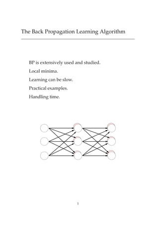
- 1. The Back Propagation Learning Algorithm BP is extensively used and studied. Local minima. Learning can be slow. Practical examples. Handling time. 1
- 2. Local Minima Algorithms based on gradient descent can become stuck in local minima. E E E wi wi wi However, generally local minima do not tend to be a problem. Speed of convergence is main problem. 2
- 3. Learning can be Slow The more layers the slower learning becomes: ¡ ¡Û Ý Ø ßÞ ´½ Ý µ Ú Ý Æ ¡Ù Æ Û Ú ´½ Ú µ Ü ßÞ Æ . . . Each error term Æ modifies the previous by a Ý ´½ Ý µ like term. Since Ý is a sigmoidal function (¼ Ý ½), then ¼ Ý´½ ݵ ¼ ¾ The more layers, the smaller the effective errors get, the slower the network learns. 3
- 4. Speeding up Learning A simple method to speeding up the learning is to add a momentum term. ¡Û ´Ø · ½µ Û · « ¡Û ´Øµ where ¼ « ½. Each weight is given some “inertia” or “momentum” so it tends to change in the direction of its average. When weight change is same every iteration (e.g. when travelling over plateau): ¡Û ´Ø · ½µ ¡Û ´Øµ ´½ «µ¡Û ´Ø · ½µ Û ¡Û ´Ø · ½µ ½ « Û So, if « ¼ , effective learning rate is ½¼ . Higher-order techniques (e.g. conjugate gradient) faster. 4
- 5. Encoder networks Momentum = 0.9 Learning Rate = 0.25 Error 10.0 0.0 0 402 Input Set[3] Output Set[0] Pat 1 Pat 1 Pat 2 Pat 2 Pat 3 Pat 3 Pat 4 Pat 4 Pat 5 Pat 5 Pat 6 Pat 6 Pat 7 Pat 7 Pat 8 Pat 8 8 inputs: local encoding, 1 of 8 active. Task: reproduce input at output layer (“bottleneck”) After 400 epochs, activation of hidden units: Pattern Hidden units Pattern Hidden units 1 1 1 1 5 1 0 0 2 0 0 0 6 0 0 1 3 1 1 0 7 0 1 0 4 1 0 1 8 0 1 1 Also called “self-supervised” networks. Related to PCA (a statistical method). Application: compression. Local vs distributed representations. 5
- 6. Example: NetTalk Sejnowski, T. & Rosenberg, C. (1986). Parallel networks that learn to pronounce English text. Complex Systems 1, 145–168. task: to convert continuous text into speech. input: a window of letters from English text drawn from a 1000 word dictionary. 7-letter context to disambiguate “brave”, “gave” vs “have” output: phonetic representation of speech (which can be fed into a synthesiser). s Hidden Units T h i s i s t h e i n p u t 6
- 7. Example: NetTalk s 26 output units 80 hidden units Hidden Units in a single layer 7 29 input units ¯ Input: letter encoded using 1 of 29 units (26 + 3 for punctuation) ¯ Output: distributed representation across 21 features including vowel height, position in mouth; 5 fea- tures for stress. Performance: 90% correct on training set. 80–87% correct on test set. Two small hidden layers better than one big layer. Babbling during learning? Hidden representations: vowel v consonants? 7
- 8. Example: Hand Written Zip Code Recognition LeCun, Y., Boser, B., Denker, J., Henderson, D., Howard, R., Hub- bard, L. & Jackel, L. (1989). Backpropagation applied to hand- written zip code recognition. Neural Computation 1, 541–551. task: Network is to learn to recognise handwritten digits taken from U.S. Mail. input: Digitised hand written numbers. output: One of 10 units is to be most active – the unit that represents the correctly recognised numeral. 8
- 9. Example: Hand Written Zip Code Recognition Real input (normalised digits from the testing set) Knowledge of task constrains architecture. “Feature detectors” useful. Implemented by weight-sharing. Reduces free parameters, speeds up learning. 9
- 10. Example: Hand Written Zip Code Recognition 0 1 2 ... 9 10 output units fully connected (310 weights) H3 ... 30 hidden units fully connected (5790 weights) 12 16 hidden units H2.1 ... H2.12 8 5 5 kernels (38592 links) from 12 H1 sets (2592 weights) 12 64 hidden units H1.1 ... H1.12 12 5 5 (19968 links) kernels (1068 weights) 16 16 digitised grayscale images Before weight sharing 64660 links After weight sharing 9760 weights 10
- 11. Example: Hand Written Zip Code Recognition Performance: error rate (%) test set training set training passes Hidden units developed spatial filters (centre-surround). Better than earlier study which used specialised hand- crafted features (Denker et al, 1989). 11
- 12. Handling temporal sequences “Spatialise” time (e.g. NetTalk) Add context units with fixed connections; some trace over time. Standard b.p. can be used in these cases. (fig 7.5 of HKP) For fully recurrent networks, b.p. extended to Real- Time Recurrent Learning (Williams & Zipser, 1989). 12
- 13. Summary Back propagation is popular training method. Hidden units find useful internal representations. Extendable to temporal sequences. Problems: can be slow, no convergence theorem. Need to try different architectures (#layers) , learning rates. Biological plausibility? 1. Who provides the targets? 2. Can signals (errors) backpropagate from one cell to another? 13