1) The document presents a process model for material recovery facilities (MRFs) that can be used in life-cycle assessments of solid waste management systems. 2) The model includes four modules for different types of MRFs that process single-stream, dual-stream, pre-sorted, and mixed waste. It estimates costs, energy use, and product flows for each type based on equipment requirements and input waste composition. 3) Results from the model show total amortized costs ranging from $19.8 to $24.9 per metric ton of waste processed across MRF types. Electricity use ranges from 4.7 to 7.8 kilowatt-hours per metric ton. Glass separation

1. Analysis of material recovery facilities for use in life-cycle assessment
Phillip N. Pressley a,⇑
, James W. Levis a
, Anders Damgaard b
, Morton A. Barlaz a
, Joseph F. DeCarolis a
a
Department of Civil, Construction, and Environmental Engineering, NC State University, 2501 Stinson Drive, Raleigh, NC 27695, USA
b
Department of Environmental Engineering, Technical University of Denmark, Miljøvej, 2800 Kongens Lyngby, Denmark
a r t i c l e i n f o
Article history:
Received 23 May 2014
Accepted 14 September 2014
Available online 7 October 2014
Keywords:
Recycling
Material recovery facility
Life-cycle assessment
Municipal solid waste
a b s t r a c t
Insights derived from life-cycle assessment of solid waste management strategies depend critically on
assumptions, data, and modeling at the unit process level. Based on new primary data, a process model
was developed to estimate the cost and energy use associated with material recovery facilities (MRFs),
which are responsible for sorting recyclables into saleable streams and as such represent a key piece
of recycling infrastructure. The model includes four modules, each with a different process flow, for sep-
aration of single-stream, dual-stream, pre-sorted recyclables, and mixed-waste. Each MRF type has a dis-
tinct combination of equipment and default input waste composition. Model results for total amortized
costs from each MRF type ranged from $19.8 to $24.9 per Mg (1 Mg = 1 metric ton) of waste input. Elec-
tricity use ranged from 4.7 to 7.8 kW h per Mg of waste input. In a single-stream MRF, equipment
required for glass separation consumes 28% of total facility electricity consumption, while all other pieces
of material recovery equipment consume less than 10% of total electricity. The dual-stream and mixed-
waste MRFs have similar electricity consumption to a single-stream MRF. Glass separation contributes a
much larger fraction of electricity consumption in a pre-sorted MRF, due to lower overall facility electric-
ity consumption. Parametric analysis revealed that reducing separation efficiency for each piece of equip-
ment by 25% altered total facility electricity consumption by less than 4% in each case. When model
results were compared with actual data for an existing single-stream MRF, the model estimated the facil-
ity’s electricity consumption within 2%. The results from this study can be integrated into LCAs of solid
waste management with system boundaries that extend from the curb through final disposal.
Ó 2014 Elsevier Ltd. All rights reserved.
1. Introduction
Life-cycle assessment (LCA) of solid waste management (SWM)
alternatives requires a modeling framework that links detailed
process-level operations within a broader system that can quantify
impacts from waste generation through final disposal and resource
recovery. The model described here has been used to develop
material recovery facility (MRF) cost and energy consumption esti-
mates for use in the Solid Waste Optimization Life-cycle Frame-
work (SWOLF), which can be used to conduct LCA that optimizes
the flow of different waste fractions within a prescribed system
boundary across a set of user-defined time stages (Levis et al.,
2013). However, the utility of such a framework depends critically
on the quality and representativeness of process-level data used to
characterize the unit processes within the system boundary. For
complex unit processes such as landfills, anaerobic digesters, or
MRFs, a single set of fixed industry-average data estimates cannot
accurately predict the performance of individual facilities that
include numerous design and operational choices and vary with
waste composition. Improved estimates require unit process mod-
els that can relate different facility configurations and input waste
compositions to changes in the resultant cost, energy consumption,
and product flows, and such process models should be designed in
a flexible manner to enable scenario exploration within a given
LCA (Laurent et al., 2014). While existing inventory databases such
as EcoInvent (2010) can provide aggregated inventory estimates
for such processes, more representative assessments require spe-
cific knowledge of constituent sub-processes informed by state-
of-the-art industry data.
The purpose of this paper is to present a detailed and novel pro-
cess model that characterizes state-of-the-art MRFs, which can be
used for life-cycle modeling of SWM systems. MRFs are an integral
part of the SWM system because they often determine the amount
of collected recyclable material that can be recovered for recycling.
Though their integration into the SWM system means that MRFs
cannot be analyzed independently of the other SWM system com-
ponents, detailed standalone MRF process models, like the one pre-
sented here, are essential to accurately model the life-cycle
impacts of full SWM systems. Recyclable materials present in
http://dx.doi.org/10.1016/j.wasman.2014.09.012
0956-053X/Ó 2014 Elsevier Ltd. All rights reserved.
⇑ Corresponding author. Tel.: +1 919 515 2331; fax: +1 919 515 7908.
E-mail address: pnpressl@ncsu.edu (P.N. Pressley).
Waste Management 35 (2015) 307–317
Contents lists available at ScienceDirect
Waste Management
journal homepage: www.elsevier.com/locate/wasman

2. municipal solid waste (MSW) have increasingly gained the atten-
tion of SWM decision makers, as recycling of MSW can contribute
to sustainability-related objectives including resource recovery,
reduced energy consumption, and lower emissions. For example,
the European waste framework directive created a 2020 recycling
target of 50% of MSW by mass for a number of fractions (EU, 2008).
In the U.S., many states and cities have instituted landfill diversion
goals. California and Florida have both set a 75% diversion target
for 2020 (California, 2012; FDEP, 2010), while cities such as San
Francisco, Oakland, and Seattle have set ‘‘zero waste’’ goals with
the intent of eliminating landfill disposal (San Francisco
Environment, 2013; Oakland, 2013; Seattle, 2013). In addition to
increased waste diversion, the environmental benefits of recycling
include the avoided use of virgin resources and energy savings
(Merrild et al., 2012).
Only limited work has been done to systematically characterize
MRF operations and the resulting emissions. Fitzgerald et al. (2012)
quantified greenhouse gas emissions at 3 MRFs to compare the
impact of dual versus single-stream facilities. However, the study
did not consider system costs and it was not clear whether the pur-
ity of recovered materials was considered, as the presence of resid-
ual materials was higher than expected. Franchetti (2009) modeled
MRF economics, but did not consider energy requirements or envi-
ronmental emissions. Chester et al. (2008) examined the total sys-
tem energy requirement and greenhouse gas emissions from
implementing recycling strategies but did not model MRFs in
detail. Themelis and Todd (2004) investigated recycling systems
used in New York City, but did not quantify environmental
impacts. With respect to MRF process models, Nishtala (1995)
developed a model that quantified MRF costs and emissions, but
it is now outdated because modern MRFs include several pieces
of automated separation equipment that were not in use 20 years
ago. Velis et al. (2013) used material flow analysis to analyze a
solid recovered fuel process that is similar to the mixed-waste
MRF modeled here. However, the input waste stream is bio-dried
and shredded, so the results are not directly comparable. None of
the aforementioned models allocate energy use and costs using a
mass balance approach. The configuration and layout of MRF-
related separation equipment depends critically on the input
stream to the facility. MRFs can be designed to accept all recycla-
bles in a single-stream, recyclables mixed with non-recyclables
(mixed waste), recyclables separated into a fiber and non-fiber
stream (dual stream), or pre-sorted recyclables. As a result, the
waste stream type accepted by the MRF determines the required
separation equipment, which in turn determines recovery efficien-
cies and energy requirements to run the equipment within the
facility, which can then be used to build a MRF life-cycle inventory.
This study builds on previous work by developing a comprehen-
sive, bottom-up model of MRFs that process (1) a single comingled
recyclables stream, (2) mixed waste, (3) dual-stream and (4) pre-
sorted recyclables. The resultant model is used to estimate MRF
energy consumption and total cost. While the development of
the MRF process model described here does not itself constitute
an LCA, it is designed to be used within an LCA framework, and
therefore needs to be informed by LCA considerations such as func-
tion, functional unit, system boundary, and allocation. Cost and
energy are tracked both because environmental performance and
cost are of interest to the recycling community, and they are
required by SWOLF, which can use the total system-wide cost of
SWM as an objective function or constraint. More broadly, we
believe that LCA should include life-cycle costing if it is to be used
to inform real world decisions that are largely driven by econom-
ics. This paper is organized as follows. Section 2 describes the mod-
eling approach, including a discussion of the assumed system
boundary and functional unit, and the data developed for this pro-
cess model, which has been obtained largely through discussions
with MRF operators and equipment vendors. Section 3 presents
results from the different MRF types and draws insights from the
analysis.
2. Materials and methods
A spreadsheet-based LCA process model was developed to rep-
resent each of the four types of MRFs described above. Major
inputs to the model include cost and energy consumption esti-
mates for each piece of MRF equipment and the separation effi-
ciencies for every modeled waste component associated with
each piece of separation equipment, which are similar to the trans-
fer coefficients used in Rotter et al. (2004) and Velis et al. (2010).
MRF performance is directly related to the composition of the
incoming waste stream, so a MRF process model should be capable
of assessing performance associated with processing each waste
component and accounting for changes to the incoming waste
stream composition (e.g., waste with a higher ferrous fraction
requires a larger magnet).
2.1. System boundaries and functional units
The system boundary for each MRF process model begins at the
tipping floor after waste is emptied from the collection vehicle. The
boundary includes the production and combustion of all fuel used
onsite, the production of all consumed electricity, and baling wire,
which is a significant cost for MRFs (Combs, 2012). The system
boundaries do not extend to the conversion of the recovered mate-
rials into new products or the offset from avoided virgin material
production. The system boundaries are narrowly drawn around
the MRFs to develop a detailed characterization of MRF life-cycle
performance, which can be incorporated into solid waste LCAs
with broader system boundaries (e.g., the entire solid waste
system).
The function of all MRFs is to separate a waste stream into
streams of saleable recyclables and a residual stream for final dis-
posal that contains non-recyclable materials and non-recovered
recyclables. The functional unit for each MRF type is 1 Mg
(1 Mg = 1 metric ton) of waste as-delivered to the MRF. Because
the composition and number of streams delivered to each MRF
type varies, the functional unit must be defined for each MRF type.
Because the functional unit differs across MRF types, direct com-
parisons of energy consumption are not meaningful. The composi-
tion of waste arriving at each MRF type is shown in Table 1. The
mixed-waste stream composition represents a complete residen-
tial waste stream. While the single-stream, dual-stream, and pre-
sorted MRF compositions are identical, the number of streams
delivered to each MRF type differs. Across these three MRF types,
we assume that recycling program participation rates and source
separation rates remain constant while only the number of waste
streams changes. The assumed composition of the waste stream
as-delivered to the MRF is based on the residential recycling com-
position of Seattle (Cascadia, 2011). The Seattle composition was
selected because it includes glass recycling, unlike ODEQ (2011),
and contaminants, unlike Beck (2005). The U.S. EPA Waste
Characterization Report (2010), which reports a recyclable stream
composition that includes all recovered materials, indicates that
OCC (old corrugated containers) represents 40% of the recovered
stream. Since most OCC is baled at commercial locations and is
not mixed with the residential waste stream, this composition
likely overestimates the significance of OCC at a MRF receiving res-
idential recyclables. However, to capture the sensitivity of results
to waste composition variation, the single-stream MRF model
was run with the ODEQ (2011), Beck (2005), and U.S. EPA (2010)
compositions to explore the sensitivity of the results to the inlet
308 P.N. Pressley et al. / Waste Management 35 (2015) 307–317

3. waste composition over a realistic range (Appendix A, Table A1).
The resulting waste composition sensitivity analysis is discussed
in Section 3.4.
2.2. Process descriptions
Each MRF is designed to recover plastic film, OCC, other fiber
such as newsprint, copy paper and third class mail, aluminum cans,
ferrous cans, plastic film, HDPE (high-density polyethylene) and
PET (polyethylene terephthalate) containers, and container glass.
Because similar equipment often has multiple names, common
U.S. industry-specific names are used throughout the description
of the process flows and all equipment is described in Table 2.
Because single-stream MRFs are common in the U.S., the single-
stream process is described first, in detail. Discussion of how other
MRF processes differ from the single-stream processes follows.
2.2.1. Single-stream process
The single-stream process flow, presented in Fig. 1, is designed
to recover fiber, glass, metals, and plastic from a commingled
recyclables stream. The equipment layout represents a general
configuration based on a review and synthesis of visits to several
single-stream MRFs currently in operation in the U.S. The collected
recyclables are unloaded from arriving trucks on the tipping floor,
where rolling stock (e.g., a front end loader) pushes material to a
drum feeder. The drum feeder distributes material to the first belt
conveyor at a constant rate, helping prevent the overload of down-
stream equipment. The first belt conveyor leads to a manual sort
where large items and materials harmful to downstream equip-
ment (e.g., wire) are removed for disposal. Additionally plastic film
(i.e., plastic bags) is recovered with a vacuum and sent to the 2-
way baler. All other materials continue to inclined Disc Screen 1
where OCC is recovered as it flows over the screen and is sent to
the 1-way baler. The unders (i.e., material that goes through the
screen) from Disc Screen 1 travel to inclined Disc Screen 2, where
newsprint is separated from containers. The unders from Disc
Screen 2, which are enriched in containers, fall on to a belt con-
veyor that leads to Disc Screen 3, which separates the remaining
fiber from the container stream. Smaller sheets of fiber flow over
Disc Screen 3, while containers and other materials fall through.
The fiber streams separated by Disc Screens 2 and 3 proceed to a
manual sort to remove contaminants before the streams are com-
bined and sent to the 1-way baler. The composition of this fiber
stream includes newsprint as well as all other fiber types accepted
by the MRF. The unders from Disc Screen 3 proceed to a glass-
breaker screen, where glass is broken into cullet, which falls
through the screen with fines. The glass and fines go to an air knife
that separates the fines and other light materials from the glass.
The glass is sent to an optical sorter, where it is sorted by color.
Table 1
Input waste composition for each MRF type.
Waste fraction Single-stream,
Dual-stream,
Pre-sorteda
Mixed-wasteb
Organics
Yard trimmings, leaves 0.0 6.7
Yard trimmings, grass 0.0 5.0
Yard trimmings, branches 0.0 5.0
Food waste – vegetable 0.0 13.8
Food waste – non-vegetable 0.0 3.5
Wood 0.0 5.0
Textiles 0.9 4.4
Rubber/leather 0.0 0.5
Fiber
Newsprint 19.5 4.9
Corr. cardboard 17.8 14.5
Office paper 0.0 2.6
Magazines 0.6 0.8
Third class mail 0.0 2.2
Mixed paper 29.7 0.0
Non-recyclable 2.7 10.5
Plastic
HDPE – translucent containers 1.1 0.4
HDPE – pigmented containers 0.0 0.7
PET – containers 2.1 1.3
Film 0.6 2.0
Non-recyclable 2.1 5.6
Metals
Ferrous cans 1.2 1.1
Ferrous metal – other 0.4 0.2
Aluminum cans 0.7 0.7
Aluminum – foil 0.2 0.2
Aluminum – other 0.0 0.0
Ferrous – non-recyclable 0.4 0.0
Aluminum – non-recyclable 0.0 0.1
Glass
Brown 5.0 2.7
Green 7.1 1.2
Clear 5.3 0.8
Non-recyclable 0.3 0.0
Miscellaneous
Organic 0.6 0.0
Inorganic 1.5 3.6
a
Single-stream, dual-stream, and pre-sorted waste compositions are based on
Seattle’s single-stream recyclable composition from Cascadia (2011).
b
Mixed-waste waste composition based on U.S. EPA (2012).
Table 2
MRF terminology descriptions.
Process Description
1-Way baler Compresses material (typically fiber) in one direction
2-Way baler Compresses material (typically containers) in two directions
Air knife Separates light materials from heavy materials via high pressure air
Drum feeder Opens bags and puts material on initial conveyor at a nearly constant rate
Eddy current
separator
Uses magnetic fields to remove aluminum and other non-ferrous metals
Negative sort Manually removes undesirable materials (contaminants); often used to purify streams of recovered materials
Optical sorter Identifies pre-determined material(s) using optical technology (e.g., cameras, lasers, sensors) and removes the identified material from the stream
using bursts of compressed air
Pickers Laborers performing manual (positive or negative) sorts in a MRF
Positive sort Pickers used to recover saleable material
Disc screen An inclined plane filled with a series of parallel rods with discs spread along each rod such that large materials travel over the top while smaller
materials fall between the discs
Glass breaker
screen
Placed several feet lower in elevation than preceding conveyor to allow gravity to break glass on screen; small pieces of glass fall through, while
larger containers go over the screen
Rolling stock Non-stationary equipment typically used to move waste on the tipping floor and bales of recovered material (e.g., front-end loader, forklift)
Tipping floor Location where trucks dump incoming waste
Trommel screen Removes smaller materials via a rotating cylindrical screen
P.N. Pressley et al. / Waste Management 35 (2015) 307–317 309

4. The color-separated glass is then subjected to a manual sort, where
ceramics and other contaminants are removed.
The overs from the glass breaker screen are conveyed to an opti-
cal sorter that recovers PET. The remaining stream is conveyed to a
second optical sorter that removes all colors of HDPE. The remain-
ing stream proceeds to a magnet for ferrous recovery. The material
remaining after the magnet proceeds to an eddy current separator
for aluminum recovery. The remaining residual stream goes to a
manual sort, where any recyclable materials missed by the separa-
tion equipment are recovered by pickers and sent to the 2-way
baler. All non-recovered material is transported offsite for final
disposal.
The aluminum, ferrous, HDPE, and PET streams are separated and
stored in cages prior to baling. Each stream is inspected for contam-
inants prior to baling. Contaminants are combined into a residual
stream that is sent offsite for final disposal. Rolling stock is used
throughout the facility to move material. Individual pieces of rolling
stock equipment are not modeled. Instead, all rolling stock fuel use is
modeled using a single coefficient in units of L fuel per incoming Mg.
Equipment separation efficiencies are presented in Table 3.
2.2.2. Mixed-waste process
The mixed-waste MRF process is identical to Fig. 1 except a
trommel screen is placed immediately after the drum feeder to
Fig. 1. Single-stream MRF process flow. This equipment configuration is used to recover aluminum, ferrous, glass, HDPE containers, mixed paper, OCC, PET containers, and
plastic film from a commingled recyclable stream. All arrows represent belt conveyors except those ending at ‘Recycling’ and ‘Residual’.
Table 3
Single-stream MRF separation efficiencies (%).a,b
Waste
fraction
Manual sort/
vacuum
Disc
Screen 1
Disc
Screen 2
Disc
Screen 3
Glass Breaker
Screen
Optical
glass
Optical
PET
Optical
HDPE
Magnet Eddy current
separator
OCC 70 85 91
Non-OCC
fiber
85 91
Plastic film 90
HDPE 98
PET 98
Fe 98
Al 97
Glass 97 98
a
Data represent the percentage of a material recovered by a given unit process. If manual separation is desired, the user can input separation efficiencies into the
appropriate manual sort option, and select manual separation instead of automated separation for the affected material. However, glass may not be separated manually.
b
Separation efficiency values were developed through expert judgment based on discussions with MRF operators and visual observation of MRF equipment during
operation.
310 P.N. Pressley et al. / Waste Management 35 (2015) 307–317

5. remove organics and fines, as shown in Appendix A, Fig. A1.
Because the MSW stream contains more contaminants (i.e., non-
recoverable materials such as food waste), equipment separation
efficiencies are lower for mixed-waste MRFs than single-stream
MRFs. Equipment separation efficiencies are presented in Appen-
dix A, Table A2.
2.2.3. Dual-stream process
Dual-stream MRFs receive separate fiber and container streams
from each collection vehicle. The dual-stream process flow is
shown in Appendix A, Fig. A2. The fiber stream in the dual-stream
MRF is processed through the three disc screens as described for a
single-stream MRF. However, the unders from Disc Screen 3 in the
dual-stream MRF are collected as residual and transported offsite
for disposal. Separation of the container stream begins with a drum
feeder and is followed by a glass breaker screen, optical sorters, a
magnet and an eddy current separator as in Fig. 1. Because the
two streams in the dual-stream MRF are treated separately, much
of the equipment in a dual-stream MRF has a smaller throughput
and capacity than a single-stream MRF for a stream with identical
mass and composition. Equipment separation efficiencies are pre-
sented in Appendix A, Table A3.
2.2.4. Pre-sorted process
Pre-sorted MRFs accept source-separated streams of OCC, mixed
paper, Al, Fe, HDPE, PET, and mixed glass. All streams except glass go
to a manual sort to remove contaminants prior to baling, as pre-
sented in Appendix A, Fig. A3. The glass stream is passed over a glass
breaker screen to break bottles into cullet, which is then passed
through an air knife for fines removal. The purified mixed glass
stream continues to an optical sorter that separates glass by color.
The glass then goes through a final manual sort to remove ceramics
or any other contaminants harmful to downstream recycling. Equip-
ment separation efficiencies are presented in Appendix A, Table A4.
2.3. Recovered material specification and separation type
The MRF process model has been developed to maximize flexi-
bility. If a material is not recovered, the equipment used to sepa-
rate it is omitted in the cost and emission calculations. For
example, if aluminum is not recovered, the eddy current separator
will be not be used. Additionally, users can override the default
configuration for a given set of recovered materials to include or
exclude any piece of modeled equipment. For example, a user
could model a mixed-waste MRF without a trommel.
To capture varying degrees of MRF automation within the
spreadsheet model, each material can be recovered manually via
pickers or automatically via separation equipment. When a mate-
rial is recovered manually, the corresponding separation equip-
ment is replaced with a positive-sort picking station. For
example, if OCC is recovered manually, Disc Screen 1, and the asso-
ciated cost and electricity consumption, is replaced by a picking
station where picker(s) recover cardboard. The only exception to
this is glass, which is always separated using a glass breaker screen
to minimize pickers’ contact with sharp broken glass. Though the
positive-sort picking station removes the same material(s) as the
equipment it replaces, the corresponding input parameter values
that describe the separation can be changed based on the presence
of manual or mechanical separation. In this analysis, all material is
recovered with automated equipment, but supplemented with
negative manual sorts for stream purification.
2.4. Mass balance
A mass balance is maintained throughout model calculations.
The mass of each material fraction passing through each piece of
equipment in each MRF type is tracked to estimate equipment
throughputs (mass per hour), which determines equipment sizing.
The separation efficiencies are organized in a matrix, like the one in
Table 3. Data on separation efficiencies have not been published, so
the values in Tables 3 and A2–A4 are based on expert judgment
resulting from discussions with MRF operators and visual observa-
tion of MRF equipment during operation.
The mass of each waste fraction, i, removed by each piece of
equipment, j, is calculated by multiplying the mass throughput
(mTP
) of j by the separation efficiency of equipment j for waste frac-
tion i, as shown in Eq. (1).
mremoved
j;i ¼ f
separation
j;i Á mTP
j;i ð1Þ
where
mremoved
j;i , mass of waste fraction i removed by equipment j (Mg),
f
separation
j;i , separation efficiency of equipment j for waste fraction i,
mTP
j;i , incoming mass to equipment j for waste fraction i (Mg).
When discussing mass throughput, we use units of mass (Mg)
and assume that the time associated with the mass flow is consid-
ered implicitly. Similarly, the mass of waste fraction i remaining
after equipment j is calculated by subtracting the mass of waste
fraction i removed by equipment j from the mass of waste fraction
i input to equipment j, as shown in Eq. (2):
mremaining
j;i ¼ mTP
j;i À mremoved
j;i ð2Þ
where
mremaining
j;i , mass of waste fraction i unaffected by equipment j (Mg).
The ‘‘mass removed’’ and ‘‘mass remaining’’ after equipment j
proceed to distinct downstream processes, as shown by the arrows
leaving each box in Fig. 1. The separation efficiency is based on the
mass removed by equipment j.
2.5. Diesel and electricity use
Diesel and/or liquefied petroleum gas (LPG) are used by rolling
stock and are input as L per incoming Mg. The diesel consumption
values used in this analysis were derived from survey results in
Combs (2012). Electricity consumption is calculated from the mass
flow to each piece of equipment, j, and the electricity demand for
equipment j per unit mass of material processed. Designed maxi-
mum equipment throughput and motor data were first used to cal-
culate electricity use per Mg throughput. To calculate the
electricity use per Mg for equipment j, the motor size was multi-
plied by the fraction of motor capacity utilized and divided by
the product of the maximum mass throughput and the fraction
of equipment capacity utilized, which accounts for equipment pro-
cessing less than maximum throughput, as shown in Eq. (3). The
fraction of motor capacity utilized accounts for motors operating
at approximately 50% of their rated capacity when a piece of equip-
ment is operating at maximum mass throughput, based on discus-
sions with equipment manufacturers.
Ej ¼ eMaxMotor
j Á f
MC
j
= mMTP
j Á f
MTP
j
ð3Þ
where
Ej, electricity requirement of equipment j (kW h per Mg),
eMaxMotor
j , motor size of equipment j,
f
MC
j , fraction of motor capacity utilized,
mMTP
j , maximum throughput mass of equipment j (Mg),
f
MTP
j , fraction of equipment capacity utilized.
The MRF model assumes a linear relationship between the
throughput of equipment j and its electricity or fuel use and cost.
For example, an eddy current separator processing two Mg of
P.N. Pressley et al. / Waste Management 35 (2015) 307–317 311

6. aluminum per hour would use twice the electricity and have dou-
ble the cost of an eddy current separator processing one Mg of alu-
minum per hour. This assumption removes the need for
specification of maximum facility throughput a priori. Therefore,
the total resource use is automatically scaled by the total Mg
throughput. In addition, the model uses the linearity assumption
to scale equipment size as waste compositions or separation effi-
ciencies are varied. For example, if the aluminum fraction in the
waste stream decreases while the PET fraction increases, the effec-
tive size of the eddy current separator will decrease because its
total throughput will decrease, while the PET optical sorter size
will increase because its total throughput will increase.
The total equipment electricity use is the sum of electricity use
for each individual piece of equipment. Additional electricity is
consumed by office use (e.g., lighting, air conditioning, computers)
and factory floor use (e.g., lighting, fans, automated doors). This
additional electricity use is allocated evenly to the material frac-
tions on a kW h per Mg basis. An explanation of equipment
resource use, including office and factory floor electricity use val-
ues, is presented in Appendix B.
Some MRFs do not have automated equipment for the separa-
tion of glass by color and plastic by type on site. Rather, they ship
separate mixtures of glass and plastic to regional sorting facilities.
The separation process is assumed to be the same whether the
sorting takes place onsite or at a centralized regional facility, thus
the electrical energy consumption is assumed to be the same. The
model allows the user to include the transportation of these mate-
rials to regional facilities, if needed.
2.6. Labor requirement calculations
MRFs employ people in several positions, including rolling stock
drivers, laborers, and supervisors. Because the hourly wage rates of
different employees may differ, labor requirements are tracked sep-
arately for each employee category. For example, the default hourly
wage rate for drivers and laborers, based on discussions with MRF
operators, is $10 and $12, respectively. Drivers are only needed to
operate rolling stock. All other non-supervisory labor is performed
by laborers. The number of supervisors is not an explicit model
input. Instead, salary for supervisors is accounted for in the man-
agement rate, expressed as a fraction of the labor rate, and assumed
to be 50% in this analysis. This management rate is combined with a
fringe benefit rate and the appropriate base wage to calculate effec-
tive wages for laborers and drivers. The labor requirement (laborer
hours per Mg throughput) associated with equipment operation
and negative sorting is calculated based on the total number of
laborers required for operation, which is an input. The value for
the total number of laborers per piece of equipment does not have
to be an integer since laborers may have duties at multiple stations
throughout the day. The number of laborers is divided by the equip-
ment throughput to calculate the total number of laborer hours
required per Mg throughput, as shown in Eq. (4).
LAE
j ¼
nlaborers
j
mMTP
j Á f
MTP
j
ð4Þ
where
LAE
j , labor requirement for equipment j in the set of automated
separation equipment and negative-sorts (laborer hours per
Mg throughput),
nlaborers
j , number of laborers required to operate equipment j,
mMTP
j , maximum throughput (MTP) mass of equipment j (Mg),
f
MTP
j , fraction of equipment capacity utilized.
When manual sorting is specified in place of automated separa-
tion, the labor requirement calculation is adjusted accordingly. The
mass removed at a positive-sorting station, which is calculated in
the mass balance, is divided by the mass of the material an individ-
ual picker can recover in an hour (i.e., the picking rate) to estimate
the labor requirement (Eq. (5)). Default picking rates for all recov-
ered materials are presented in Appendix A, Table A5.
LMPS
j ¼
mremoved; total
j
mTP
j Á rpicking
j
ð5Þ
where
LMPS
j , labor requirement for picking station j in the set of manual
positive sorts (MPS) (laborer hours per Mg throughput),
mremoved; total
j , total mass removed at picking station j (Mg),
mTP
j , throughput mass of picking station j (Mg),
rpicking
j , picking rate associated with equipment j (For example, a
positive sort targeting aluminum would have an aluminum
picking rate.) (Mg material per laborer hour).
The total facility laborer requirement is calculated in a similar
manner to the total facility electricity use. The laborer requirement
per Mg of material processed by equipment j is multiplied by the
throughput of equipment j. The equipment-specific laborer
requirements are then summed over all pieces of MRF equipment.
The facility driver requirement is calculated following the same
procedure.
2.7. Cost estimation
This model uses capital, material, and labor cost data along with
the calculated mass balance, labor requirements, and resource con-
sumption to estimate the total cost per unit input mass using Eq.
(6):
Ctotal
¼ CNEC
þ CEq
þ CL
þ CR
ð6Þ
where
Ctotal
, total amortized cost ($),
CNEC
, non-equipment amortized capital cost ($),
CEq
, amortized equipment cost ($),
CL
, labor cost ($),
CR
, resource cost ($).
The amortized cost, in U.S. dollars ($) per Mg summed over all
waste fractions, is calculated from the capital costs for building
construction and equipment purchase as well as the annual costs
for personnel, diesel and electrical energy, and other operating
costs (Eq. (6)). The capital costs associated with equipment and
building acquisition are amortized, or converted from a single
lump sum cost in the first year to an annual cost over the MRF life-
time, using a 5% discount rate and an estimated equipment life-
time, shown in Table 4. The amortized building and land costs
are summed to represent the non-equipment capital cost, CNEC
.
The amortized equipment capital cost and annual equipment
maintenance cost are summed to represent the total equipment
cost, CEq
, as shown in Appendix B, Equation B5. The labor cost, CL
,
includes the general labor cost and driver cost, with supervision
and fringe multipliers, as shown in Appendix B, Equation B8. The
resource cost, CR
, includes the cost of electricity and diesel used
within the facility and the cost of wire to bale recovered materials.
Appendix B.2 presents calculations for each term in Eq. (6).
2.8. Allocation
Total costs and energy consumption are allocated to individual
waste fractions so that model performance is responsive to waste
composition. Furthermore, optimization of waste flows through a
solid waste system, as in SWOLF, requires energy and costs to be
312 P.N. Pressley et al. / Waste Management 35 (2015) 307–317

7. allocated to individual waste components to determine the opti-
mal technology choices and mass flows through an integrated solid
waste system. For example, given a specific model objective (e.g.,
minimize GHG emissions), SWOLF calculates whether recycling
paper to avoid virgin paper production is preferable to landfilling
paper or combustion with energy recovery. Thus, all energy and
costs must be allocated to individual waste fractions.
The allocation method is mass-based and varies based on the
attributes of the equipment. For equipment that is used to remove
and recover one or more waste fractions, the resource use and cost
for the total throughput are allocated to only the removed materi-
als. For example, the magnet and eddy current separator energy
consumption and costs are allocated only to ferrous and alumi-
num, respectively, because those are the materials in the waste
composition that necessitate the use of that equipment. In con-
trast, some equipment separates two streams that contain recover-
able materials (i.e., disc screens, glass breaker screens). In this case,
costs and resource use are allocated to the total throughput. For
equipment that does no separation (i.e., drum feeders, balers, roll-
ing stock), the allocation is also based on total throughput. Future
analyses may require allocation of resource use and cost to streams
different than those presented here (e.g., combustibles to waste-
to-energy), so the model allows the user to allocate resource use
and cost to the equipment’s input stream, the residual output
stream, or the product output streams.
2.9. Development of model input data
Information on the cost, capacity, and energy consumption for
each piece of equipment was obtained through contact with
vendors and MRF operators as summarized in Combs (2012).
Discussions with MRF operators and equipment vendors were
required to document current state-of-the-art technology and
facility configuration. A complete list of model input data is pre-
sented in Appendix C.
3. Results and discussion
To examine MRF cost and performance, the model was used to
calculate mass flows, energy requirements, and cost per unit mass
input for each MRF type. The mass flows were used to calculate
recovery rates for all recyclable materials, which are important in
solid waste LCAs that consider downstream processing of sorted
waste. Electricity and rolling stock fuel requirements were calcu-
lated, which can be used to estimate the associated emissions.
Total facility costs were estimated for each MRF type. Sensitivity
analysis on equipment separation efficiencies and waste composi-
tion was performed for the single-stream MRF. Though four MRF
types are presented in this analysis, meaningful direct comparison
across MRF types is inappropriate because the mixed waste MRF
has a different functional unit, owing to the different waste compo-
sition it accepts relative to the others. Though not modeled in this
analysis, different waste collection schemes must be considered to
account for differences in upstream waste flow.
3.1. Material recovery rates for each MRF type
Using the mass balances from each MRF model and the
assumed separation efficiencies, recovery rates for all recycled
materials were derived and are shown in Table 5. Metal recovery
rates are the highest, with recoveries ranging from 87% to 100%
for aluminum and ferrous. OCC is recovered at a higher rate than
Table 4
Throughput, energy requirement, cost, and labor data for each piece of automated equipment (based on Combs (2012)).
Equipment Max
throughput
(Mg/h)
Fraction of
equipment
capacity
utilized
Fraction of
motor rated
capacity
utilized
Rated
motor
capacity
(kW)
Diesel
use
(L/Mg)
Investment
cost ($)
Fixed
OM
costa
($/yr)
Number of Laborers
required for max.
throughput
Number of
drivers
required
Lifetime
(yr)
Conveyor 30 0.85 0.5 5.6 0 46,000 10,000 0 0 10
Drum feeder 30 1 0.5 15 0 150,000 100 0 0 10
Vacuum 10 0.85 0.5 5 0 150,000 100 2 0 10
Disc Screen 1 45 0.85 0.5 8.5 0 175,000 10,000 0 0 10
Disc Screen 2 21 0.85 0.5 5.5 0 400,000 13,000 0 0 10
Disc Screen 3 7 0.85 0.5 10 0 280,000 10,000 0 0 10
1-Way baler 51 1 0.5 63 0 550,000 5000 1 0 10
Glass breaker
screen
9 0.85 0.5 30 0 220,000 10,000 0 0 10
Air knife 36 0.85 0.5 164 0 62,500 10,000 0 0 10
Optical glass 5 0.95 0.5 69 0 825,000 30,000 0 0 10
Optical PET 10 0.85 0.5 13 0 225,000 5000 0 0 10
Optical HDPE 10 0.85 0.5 40 0 450,000 10,000 0 0 10
Magnet 2 0.85 0.5 4 0 35,000 5000 0 0 10
Eddy current
separator
12 0.85 0.5 9 0 128,000 5000 0 0 10
2-Way baler 30 1 0.5 59 0 530,000 5000 1 0 10
Trommel 45 0.85 0.5 62 0 125,000 10,000 0 0 10
Rolling stock 24 0.85 – – 10 350,000 5000 0 1 10
a
OM = operations and maintenance.
Table 5
Calculated recovery and residual rates by MRF type and material (%). Though the single-stream, dual-stream, and pre-sorted MRFs have similar recovery rates, the high
contaminant rate in the mixed-waste MRF reduces recovery efficiency and increases the residual rate.
MRF type OCCa
Non-OCC fiber Al Fe Film HDPE PET Glass Residual rateb
Single-stream 100 99 97 98 90 98 98 95 10
Mixed-waste 76 39 87 88 77 83 83 69 76
Dual-stream 99 98 96 97 0 97 97 93 11
Pre-sorted 100 100 100 100 0 100 100 95 2
a
OCC recovery rate includes OCC removed by Disc Screens 2 and 3 that is baled as mixed paper.
b
Residual rate represents the percentage of incoming waste that is not recovered and requires additional downstream treatment.
P.N. Pressley et al. / Waste Management 35 (2015) 307–317 313

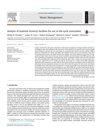
8. non-OCC fiber in all MRF types. Mixed-waste MRFs have a lower
fiber recovery rate because high contamination rates reduce sepa-
ration efficiencies. HDPE and PET have similar recovery rates, rang-
ing from 83% to 100%. Glass recovery rates range from 93% to 95%,
except in the mixed-waste MRF, where a trommel removes some
broken glass with the organic fraction, lowering the recovery rate
to 69%. The pre-sorted MRF removes fewer contaminants from
input waste streams, which reduces the percentage of input mass
that is not recovered (i.e., residual rate) below those in the dual-
stream and single-stream MRFs. The dual-stream recovery rates
are lower than the single-stream rates because the fiber stream
is assumed to contain 1% of the container stream and vice versa.
This contamination also increases the dual-stream MRF’s residual
rate.
Because the mixed-waste MRF has a different input waste com-
position, its recovery rates are not directly comparable to the other
MRF types. Since there is no source-separation of recyclables prior
to arrival at the mixed-waste MRF, 76% of the input mass is resid-
ual. Recovery rates for all MRF types reflect the fraction of material
recovered from the waste stream sent to the MRF based on the
default compositions given in Table 1.
3.2. Resource use for each MRF type
Electricity, diesel, and baling wire consumption were quantified
for each MRF type. The model can accommodate LPG rolling stock,
but only diesel rolling stock is included in this analysis. Though
diesel use is shown in Table 6, the rolling stock diesel requirement
per Mg is a model input, as noted in Section 2.5. The data used for
each MRF type are based on single-stream MRF survey results
(Combs, 2012). Wire use is inversely correlated to the residual
rates. Higher residual rates cause low wire consumption per Mg
of waste input since the residuals are not baled. Thus, the pre-
sorted MRF requires more wire per Mg, since only 2% of the each
input Mg is residual. Note that if waste composition changes such
that the fraction of lighter recyclable materials (i.e., plastics)
increases, wire requirements per Mg would likely increase because
the wire requirement per mass of baled material is relatively high
for plastics given their lower density.
Electricity use is highest in the mixed-waste MRF because a lar-
ger mass of contaminants is carried through the system, requiring
larger equipment capacities to process the extra material. Since the
fiber separation equipment does not have to accommodate the
container stream in the dual-stream MRF, it uses less electricity
than in the single-stream MRF. The pre-sorted MRF electricity
use is much less than the other MRFs due to the limited amount
of separation equipment. However, the input streams to the pre-
sorted MRF are likely a result of curbside sorting, which consumes
more fuel than other collection schemes. Thus, integrated analyses
of SWM systems are required to quantify relative environmental
performance of alternatives for recyclable recovery.
Examination of electricity consumption allocated to each recov-
ered material reveals large variations in resource consumption by
material. However, electricity use is a result of both separation
technology and the fraction of the material in the final residual
stream. Table 7 shows that per material electricity consumption
generally follows total MRF electricity consumption, with the high-
est values for a mixed-waste MRF. HDPE recovery uses more elec-
tricity than all other materials, due to the high energy use per Mg
of the HDPE optical sorter, in all MRFs except the pre-sorted MRF,
which does not include an HDPE optical sorter. Ferrous recovery
requires more electricity than aluminum recovery, except in the
pre-sorted MRF where consumption is equal, due to separation
using identical conveyors, manual sorts, and balers, that employs
neither a magnet nor an eddy current separator. Because OCC,
non-OCC fiber, and film are removed early in the process via equip-
ment with relatively low electricity consumption, they use less
electricity than other materials. Note all values in Table 7 have
been normalized to the mass of material input. These values must
be combined with a waste composition to calculate MRF resource
use values.
Equipment electricity consumption varies based on throughput
and motor size. The glass optical sorter and air knife, which are
required for glass separation, consume 28% of the total single-
stream MRF electricity for the default composition, as shown in
Fig. 2. Disc screens, which separate fiber, consume less than 10%
of MRF electricity, as do the plastic optical sorters. The magnet
and eddy current separator are responsible for only 3% of MRF elec-
tricity consumption. Thus, a decrease in the glass fraction will
result in greater reductions to total single-stream MRF electricity
consumption than comparable decreases in other waste fractions.
Electricity consumption by equipment for all MRFs is in Appendix
A Table A6.
Several previous studies have reported MRF resource consump-
tion and cost. Fitzgerald et al. (2012) found 0.8 and 0.7 L per Mg of
diesel consumption in dual-stream and single-stream MRFs,
Table 6
Resource use for each MRF type. More automation in the mixed-waste MRF causes higher electricity consumption. The low residual and limited automation of the pre-sorted MRF
result in larger wire consumption and lower electricity consumption.
MRF type Electricity (kW h/Mginput) Diesel (L/Mginput) Wire mass (kg/Mginput)
Single-stream 6.2 0.7 0.6
Mixed-waste 7.8 0.7 0.3
Dual-stream 6.0 0.7 0.6
Pre-sorted 4.7 0.7 0.7
Table 7
Electricity consumption (kW h per Mg material) by recovered material in each MRF type. Materials (i.e., glass, HDPE, PET) removed via equipment with high electricity demands
(i.e., optical sorters) have higher electricity consumption, as do materials that travel farther through the process (i.e., aluminum and ferrous).
Recovered material Single-stream Mixed-waste Dual-stream Pre-sorted
OCC 2.6 4.7 3.4 2.7
Non-OCC fiber 3.0 5.4 3.8 2.7
Aluminum 9.7 28.1 6.1 3.1
Ferrous 11.7 52.0 7.8 3.1
Film 3.0 4.7 2.1 3.1
HDPE 32.7 116.1 22.0 3.1
PET 9.9 36.9 6.9 3.1
Glass 16.8 36.4 14.8 14.0
314 P.N. Pressley et al. / Waste Management 35 (2015) 307–317

9. respectively, which are comparable to the consumption values
used in this analysis (Table 6). Fitzgerald et al. (2012) also reported
electricity consumption of 11.5 and 13.8 kW h per Mg for the dual-
stream and single-stream MRFs, respectively, which are approxi-
mately double the values calculated in this analysis. The discrep-
ancy in electricity consumption may be the result of increasing
economies of scale, since most of the MRFs surveyed for this study
were larger than those in the Fitzgerald study. Furthermore, the
level of automation and type of lighting used in the Fitzgerald
study is unknown. Chester et al. (2008) presents electricity con-
sumption values comparable to the results of this study, but the
Chester MRFs have less automation. However, Chester’s MRFs have
less than 25% of the mass throughput of the MRFs surveyed in
Combs (2012), which were adapted for this analysis. The lighting
estimate used for the operating floor in this analysis represents
energy efficient T5 fluorescent bulbs, which consume 7% of total
single-stream MRF electricity.
3.3. Costs for each MRF type
The cost per Mg input for each MRF type includes costs for the
purchase and maintenance of equipment, labor, wire, fuel, electric-
ity, and the capital costs associated with land procurement and
building construction. The largest fraction of the total cost is the
capital cost of land procurement and building construction, which
ranges from 49% to 62% of the total cost. Of course, both of these
factors will vary with location. Land procurement and building
construction are the same between MRF types because the same
land and construction data were used. The equipment costs range
from 17%, for the pre-sorted MRF with less separation equipment,
to 32% of total cost, for the mixed-waste MRF that must have larger
equipment to handle the large residual fraction throughout. The
labor costs for single-stream and dual-stream MRFs, shown in
Table 8, are much larger than the $1.7 and $1.5 per Mg for
mixed-waste and pre-sorted MRFs respectively. The mixed-waste
MRF labor cost per unit mass is much lower because labor costs
are distributed over a larger quantity of waste. The labor costs
are smaller in a pre-sorted MRF because less separation is required
relative to the other MRF types. The wire costs in Table 8 are
directly proportional to wire consumption presented in Table 6
and have been included here because they contribute up to 8% of
the total cost.
The single-stream MRF has the highest total cost of $24.9 per
Mg input. The dual-stream MRF is less expensive to operate, in
part, because processing two streams allows the fiber separation
equipment that is placed early in the single-stream process to be
smaller in a dual-stream MRF. Though the mixed-waste MRF has
much larger equipment costs, the smaller labor and wire costs
result in a total unit cost that is less than the single-stream MRF.
Of course, the total throughput and mass of residuals are consider-
ably higher for a mixed waste MRF. The pre-sorted MRF is less
complex, resulting in the lowest equipment, labor, fuel, and elec-
tricity costs.
MRF costs have been previously explored, but they focus on
small MRFs with little automation and high labor requirements.
Thus, many of these costs are higher than the costs presented in
this analysis. Chester et al. (2008) reported capital and mainte-
nance costs ranging from 10% to 30% greater than this analysis
but comparable electricity values. Franchetti (2009) has total
dual-stream MRF costs 90% greater than the costs presented here,
largely due to the representation of a more labor intensive process.
3.4. Parametric analysis of waste composition and equipment
separation efficiencies in a single-stream MRF
To explore model response to different waste compositions, the
single-stream model was run with the default and three additional
waste compositions as given in Appendix A, Table A1. The default
waste composition, from Cascadia (2011), quantifies the composi-
tion of the household-separated recyclable stream in Seattle,
Washington. Contaminants make up 5.9% of the incoming waste.
Beck (2005) reported the statewide commingled recycling stream
composition for Pennsylvania. No contaminants were included in
the composition. ODEQ (2011) reported residential commingled
recyclable composition, which is influenced by the fact that con-
tainer glass as well as plastic and aluminum containers have
deposits and are partially recovered outside of the residential recy-
clable stream. This explains the relatively low (1.4%) glass content
in the ODEQ recyclables stream. Because the purpose of this sensi-
tivity analysis is to explore model response to waste composition
variation, the model recovered glass and film for all waste compo-
sitions, though glass and film would probably not be recovered for
compositions like ODEQ (2011). Other contaminants in the ODEQ
(2011) composition made up 5.7% of the incoming mass, which is
the sum of the non-recyclable paper, non-recyclable plastic, and
miscellaneous inorganics in Appendix A, Table A1. U.S. EPA
(2010) was used to estimate a commingled recyclables composi-
tion, by combining masses of recovered materials. This composi-
tion does not isolate the residential stream, so 40% of the mass is
OCC. Like Beck (2005), no contaminants are included in this waste
composition, so the resulting residual rate is much lower than
Fig. 2. Sensitivity of single-stream MRF electricity use to waste composition.
Table 8
Cost summary by MRF type. The single-stream MRF has the highest total cost because of its relatively high equipment and labor costs, while the low equipment and labor costs in
a pre-sorted MRF contribute to its low total cost.
MRF type Total equipment cost
($/Mg input)
Labor
($/Mg input)
Wire Cost
($/Mg input)
Fuel and electricity cost
($/Mg input)
Building and land capital costs
($/Mg input per year)
Total costs
($/Mg input)a
Single-stream 5.8 4.3 1.3 1.3 12.3 24.9
Mixed-waste 7.7 1.7 0.5 1.5 12.3 23.6
Dual-stream 5.3 3.3 1.2 1.3 12.3 23.4
Pre-sorted 3.3 1.5 1.5 1.2 12.3 19.8
a
Individual values may differ slightly from the total due to rounding.
P.N. Pressley et al. / Waste Management 35 (2015) 307–317 315

10. residuals for the ODEQ (2011) and Cascadia (2011) streams. Elec-
tricity consumption under all four waste compositions is provided
in Fig. 2.
The effect of waste composition on electricity consumption and
cost is presented in Table 9 and Fig. 2. The changes in cost are a
result of changes to equipment as well as changes to electricity
and wire consumption. The costs for the different waste composi-
tions are within 7% of the average, which is likely well within the
model uncertainty. Though the ODEQ (2011) composition has a
large residual rate, its electricity consumption and total cost are
less than the other waste compositions. Much of the comparative
savings can be attributed to decreased size and electricity con-
sumption of the glass breaker screen and glass optical sorter, as
shown in Fig. 2. Beck (2005) has the highest electricity consump-
tion due in part to its high glass content (21%), which increases
the electricity consumption by the glass breaker screen and glass
optical sorter. Baler electricity use per Mg is smaller because the
Beck composition includes contaminants as well as glass, which
results in more unbaled material than the other MRF types.
To explore the effects of separation efficiencies on electricity
consumption within a single-stream MRF, the separation efficien-
cies for sorting equipment were altered one piece of equipment
at a time, by subtracting 25% from all non-zero separation efficien-
cies, as presented in Appendix A Table A7. The percent change in
electricity compared to the default electricity consumption was
used as a metric to examine the relative impact of each piece of
equipment’s separation efficiency values (Fig. 3).
When the separation efficiency of the glass breaker screen is
reduced, more glass contaminates the containers stream, which
necessitates increasing the size of equipment meant to separate
containers. However, this increase in equipment size is offset by
the reduction in downstream equipment size and thus electricity
demand due to the decreased throughput of the air knife and glass
optical sorter. Reducing the separation efficiencies of a glass
breaker screen by 25% results in a 3.6% decrease in single-stream
MRF electricity consumption. As the separation efficiency of a disc
screen decreases, additional paper goes to downstream equipment,
and the increased electricity demand of downstream equipment
exceeds the savings at the disc screen. Disc Screen 2 produces
the largest change among the disc screens because it is the first
screen to process the non-OCC fiber stream, and it processes the
30% of OCC not removed by Disc Screen 1. Reducing the PET optical
sorter separation efficiencies slightly increases the electricity
demand because of increased downstream equipment size. The
effect of changing any other equipment’s separation efficiencies
results in a change to total electricity consumption less than
0.1%, which is less than the precision of the model. While changes
in separation efficiency do not have a significant effect on MRF per-
formance, they may have a large impact on the performance of
downstream processes, which are not accounted for in this analy-
sis. For example, higher levels of contaminants in the paper stream
can affect the paper recycling process by limiting the type and
quality of recycled paper that can be produced from it (Miranda
et al., 2013).
3.5. Comparison with operating MRF
To evaluate the MRF model described here, electricity consump-
tion from an operating MRF was compared with estimates from the
single-stream MRF model. Model inputs were adjusted to match
the equipment layout and facility size of the actual MRF described
in Combs (2012) as closely as possible. Additionally, the lighting
electricity use from Combs (2012) was used because the model
defaults are for energy efficient fluorescent lighting, which was
not installed at the surveyed MRF. Input waste composition data
was not available for the operating MRF, so the default composi-
tion from Table 1 was used. The model estimates electricity con-
sumption to be 24.3 kW h per Mg, while the actual MRF
consumption was 23.8 kW h per Mg. Thus, the model overesti-
mated the MRF’s electricity consumption by only 2%.
As shown in Table 9, when the model is used with default val-
ues, MRF electricity consumption is estimated to be 6.2 kW h per
Mg, which is nearly a factor of 4 lower than the estimate for the
actual MRF discussed above. The default values assume modern
lighting and small office space, which each contribute 8% of total
MRF electricity use, but the surveyed MRF was modeled with large
office space and older lighting, which contributed 17% and 69% of
the total MRF electricity use, respectively. These results serve to
emphasize the importance of a MRF process model that is respon-
sive to waste composition, process flow, and facility design (e.g.,
lighting technology).
3.6. Conclusions
The model presented here quantifies MRF cost and energy con-
sumption over a broad set of conditions. The MRF model represents
a significant improvement over fixed estimates of MRF electricity
consumption, since MRF performance can vary significantly
depending on facility design and incoming waste composition.
The model can also allocate electricity use to each waste fraction,
enhancing the capability of SWM LCA models such as SWOLF.
The model described here is the first to both represent a modern
automated MRF and respond to changes in MRF facility design.
The results show that resource demands and costs associated
with MRF operation vary by both MRF type and input waste com-
position. The electricity use associated with glass separation equip-
ment is greater than all other types of separation equipment. Thus,
Table 9
Model response to variations in waste composition in a single-stream MRF.
Result Cascadia (2011) ODEQ (2011) Beck (2005) U.S. EPA (2010)
Residual rate (%) 10 9 2 2
Electricity consumed (kW h/Mg) 6.2 4.2 7.0 5.4
Total cost ($/Mg) 24.9 23.9 26.6 24.3
Fig. 3. Parametric sensitivity analysis for a 25% decrease in separation efficiencies
for selected equipment within a single-stream MRF. MRF equipment is ordered
from top (largest effect) to bottom (smallest effect).
316 P.N. Pressley et al. / Waste Management 35 (2015) 307–317

11. energy efficiency gains associated with the glass separation tech-
nology will result in larger reductions in facility electricity con-
sumption than any other equipment. The floor area per Mg of
facility throughput and the installed lighting technology in the sep-
aration area have the potential to impact total facility electricity
consumption. Because of the small contribution of resource use
to total cost, increased electrical and fuel efficiency will not signif-
icantly affect MRF costs. Due to high capital costs, varying waste
composition resulted in small changes to total costs in the sin-
gle-stream MRFs. However, the range in electricity consumption
in response to variations in waste composition was more than
40% of the baseline electricity consumption. Though there is uncer-
tainty in separation efficiencies, sensitivity analysis revealed large
reductions to individual equipment separation efficiencies resulted
in only small changes in total electricity consumption within the
MRF, though potential downstream effects were not quantified.
Narrow system boundaries were purposely established in this
analysis to isolate MRF cost and performance. This model and asso-
ciated results can be integrated into LCAs with broader system
boundaries to evaluate waste management from curbside collec-
tion through final disposal. Though pre-sorted MRFs ostensibly
appear to be cheaper, less energy-intensive, and less GHG intensive
than other MRF types, MRF performance must be considered in the
context of the larger solid waste management system. For exam-
ple, pre-sorted MRFs typically receive the separated streams from
systems with curbside separation, which results in higher collec-
tion fuel consumption and cost compared to single-stream collec-
tion. Consideration of waste collection options associated with
each MRF type, disposal options for residual waste, and avoided
emissions associated with the recovered materials are important
considerations in any integrated systems analysis of solid waste
management.
Acknowledgements
This research was supported by the National Science Founda-
tion and the Environmental Research and Educational Foundation.
Appendix A. Supplementary data
Supplementary data associated with this article can be found, in
the online version, at http://dx.doi.org/10.1016/j.wasman.2014.
09.012.
References
Beck, R.W., 2005. Pennsylvania Recovered Material Composition Study.
Cascadia (Consulting Group), 2011. Residential Recycling Stream Composition
Study Final Report.
Chester, M., Martin, E., Sathaye, N., 2008. Energy, greenhouse gas, and cost
reductions for municipal recycling systems. Environ. Sci. Technol. 42, 2142–
2149.
(City of) Oakland, 2013. OaklandRecycles. http://www2.oaklandnet.com/
Government/o/PWA/o/FE/s/GAR/OAK024364.
(City of) Seattle, 2013. Zero Waste Strategy. http://www.seattle.gov/council/
issues/zerowaste.htm.
Combs, A.R., 2012. Life-Cycle Analysis of Recycling Facilities in a Carbon
Constrained World. North Carolina State University, Raleigh, North Carolina,
United States. http://repository.lib.ncsu.edu/ir/bitstream/1840.16/7808/1/
etd.pdf.
Ecoinvent Data V2.2, 2010. Swiss Centre for Life-cycle Inventories.
EU (European Union), 2008. Directive 2008/98/EC of the European Parliament and
of the Council of 19 November 2008 on waste and repealing certain Directives
Text with EEA relevance. Official J. 312, 0003–0030.
FDEP (Florida Department of Environmental Protection), 2010. 75% Recycling goal
report to legislature. http://www.dep.state.fl.us/waste/quick_topics/
publications/shw/recycling/75percent/75_recycling_report.pdf.
Fitzgerald, G.C., Krones, J.S., Themelis, N.J., 2012. Greenhouse gas impact of dual
stream and single stream collection and separation of recyclables. Resour.,
Conservation Recycl. 69, 50–56.
Franchetti, M.J., 2009. Case study: determination of the economic and operational
feasibility of a material recovery facility for municipal recycling in Lucas
County, Ohio, USA. Resour., Conservation Recycl. 53, 535–543.
Laurent, A., Clavreul, J., Bernstad, A., Bakas, I., Niero, M., Gentil, E., Christensen, T.H.,
Hauschild, M.Z., 2014. Review of LCA studies of solid waste management
systems – part II: methodological guidance for a better practice. Waste Manage.
34, 589–606.
Levis, J.W., Barlaz, M.A., DeCarolis, J.F., Ranjithan, S.R., 2013. A generalized
multistage optimization modeling framework for life-cycle assessment-based
integrated solid waste management. Environ. Modell. Softw. 50, 51–65.
Merrild, H., Larsen, A.W., Christensen, T.H., 2012. Assessing recycling versus
incineration of key materials in municipal waste: the importance of efficient
energy recovery and transport distances. Waste Manage. 32, 1009–1018.
Miranda, R., Monte, M.C., Blanco, A., 2013. Analysis of the quality of the recovered
paper from commingled collection systems. Resour., Conservation Recycl. 72,
60–66.
Nishtala, S.R., 1995. Design and Analysis of Material Recovery Facilities in an
Integrated Solid Waste Management System. North Carolina State University,
Raleigh, North Carolina, United States.
ODEQ (Oregon Department of Environmental Quality), S.W.P. and P.D.S.L.Q.D., 2011.
Composition of Commingled Recyclables Before and After Processing.
Rotter, V.S., Kost, T., Winkler, J., Bilitewski, B., 2004. Material flow analysis of RDF-
production processes. Waste Manage. 24, 1005–1021. http://dx.doi.org/
10.1016/j.wasman.2004.07.015.
San Francisco Environment, 2013. Zero Waste Website. http://
www.sfenvironment.org/zero-waste.
(State of) California, 2012. California’s new goal: 75% recycling. CalRecycle. http://
www.calrecycle.ca.gov/75percent/Plan.pdf.
Themelis, N.J., Todd, C.E., 2004. Recycling in a megacity. J. Air Waste Manage Assoc.
54, 389–395.
U.S. EPA (United States Environmental Protection Agency), 2010. Municipal Solid
Waste Generation, Recycling, and Disposal in the United States: Facts and
Figures for 2009.
U.S. EPA (United States Environmental Protection Agency), 2012. Municipal Solid
Waste Generation, Recycling, and Disposal in the United States: Facts and
Figures for 2011.
Velis, C.A., Longhurst, P.J., Drew, G.H., Smith, R., Pollard, S.J.T., 2010. Production and
quality assurance of solid recovered fuels using mechanical—biological
treatment (MBT) of waste: a comprehensive assessment. Crit. Rev. Environ.
Sci. Technol. 40, 979–1105. http://dx.doi.org/10.1080/10643380802586980.
Velis, C.A., Wagland, S., Longhurst, P., Robson, B., Sinfield, K., Wise, S., Pollard, S.,
2013. Solid recovered fuel: materials flow analysis and fuel property
development during the mechanical processing of biodried waste. Environ.
Sci. Technol. 47, 2957–2965. http://dx.doi.org/10.1021/es3021815.
P.N. Pressley et al. / Waste Management 35 (2015) 307–317 317