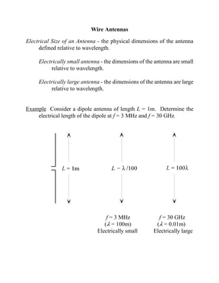
1. Wire Antennas
Electrical Size of an Antenna - the physical dimensions of the antenna
defined relative to wavelength.
Electrically small antenna - the dimensions of the antenna are small
relative to wavelength.
Electrically large antenna - the dimensions of the antenna are large
relative to wavelength.
Example Consider a dipole antenna of length L = 1m. Determine the
electrical length of the dipole at f = 3 MHz and f = 30 GHz.
f = 3 MHz f = 30 GHz
(8 = 100m) (8 = 0.01m)
Electrically small Electrically large

2. Infinitesimal Dipole
()l . 8/50, a << 8)
We assume that the axial current along the infinitesimal dipole is
uniform. With a << 8, we may assume that any circumferential currents
are negligible and treat the dipole as a current filament.
The infinitesimal dipole with a constant current along its length is a non-
physical antenna. However, the infinitesimal dipole approximates several
physically realizable antennas.

3. Capacitor-plate antenna (top-hat-loaded antenna)
The “capacitor plates” can be actual conductors or simply the wire
equivalent. The fields radiated by the radial currents tend to cancel each
other in the far field so that the far fields of the capacitor plate antenna can
be approximated by the infinitesimal dipole.
Transmission line loaded antenna
If we assume that L . 8/4, then the current along the antenna resembles
that of a half-wave dipole.

4. Inverted-L antenna
Using image theory, the inverted-L antenna is equivalent to the
transmission line loaded antenna.
Based on the current distributions on these antennas, the far fields of the
capacitor plate antenna, the transmission line loaded antenna and the
inverted-L antenna can all be approximated by the far fields of the
infinitesimal dipole.

5. To determine the fields radiated by the infinitesimal dipole, we first
determine the magnetic vector potential A due to the given electric current
source J (M = 0, F = 0).
The infinitesimal dipole magnetic vector potential given in the previous
equation is a rectangular coordinate vector with the magnitude defined in
terms of spherical coordinates. The rectangular coordinate vector can be
transformed into spherical coordinates using the standard coordinate
transformation.

6. The total magnetic vector potential may then be written in vector form as
Because of the true point source nature of the infinitesimal dipole ()l .
8/50), the equation above for the magnetic vector potential of the
infinitesimal dipole is valid everywhere. We may use this expression for
A to determine both near fields and far fields.
The radiated fields of the infinitesimal dipole are found by
differentiating the magnetic vector potential.

8. The electric field is found using either potential theory or Maxwell’s
equations.
Potential Theory
Maxwell’s Equations (J = 0 away from the source)
Note that electric field expression in terms of potentials requires two levels
of differentiation while the Maxwell’s equations equation requires only one
level of differentiation. Thus, using Maxwell’s equations, we find

9. fields radiated by an
infinitesimal dipole

10. Field Regions of the Infinitesimal Dipole
We may separate the fields of the infinitesimal dipole into the three
standard regions:
³ Reactive near field kr << 1
´ Radiating near field kr > 1
µ Far field kr >> 1
5
4.5
4
3.5
3
2.5
2
1.5
1
0.5
0
0 2 4 6 8 10 12
Considering the bracketed terms [ ] in the radiated field expressions for the
infinitesimal dipole ...
³ Reactive near field (kr << 1) (kr)-2 terms dominate
´ Radiating near field (kr > 1) constant terms dominate if present
otherwise, (kr)-1 terms dominate
µ Far field (kr >> 1) constant terms dominate

11. Reactive near field [ kr << 1 or r << 8/2B ]
When kr << 1, the terms which vary inversely with the highest power
of kr are dominant. Thus, the near field of the infinitesimal dipole is given
by
Infinitesimal dipole
near fields
Note the 90o phase difference between the electric field components and
the magnetic field component (these components are in phase quadrature)
which indicates reactive power (stored energy, not radiation). If we
investigate the Poynting vector of the dominant near field terms, we find
The Poynting vector (complex vector power density) for the infinitesimal
dipole near field is purely imaginary. An imaginary Poynting vector
corresponds to standing waves or stored energy (reactive power).

12. The vector form of the near electric field is the same as that for an
electrostatic dipole (charges +q and !q separated by a distance )l).
If we replace the term (Io0/k) by in the near electric field terms by its
charge equivalent expression, we find
The electric field expression above is identical to that of the electrostatic
dipole except for the complex exponential term (the infinitesimal dipole
electric field oscillates). This result is related to the assumption of a
uniform current over the length of the infinitesimal dipole. The only way
for the current to be uniform, even at the ends of the wire, is for charge to
build up and decay at the ends of the dipole as the current oscillates.
The near magnetic field of the infinitesimal dipole can be shown to
be mathematically equivalent to that of a short DC current segment
multiplied by the same complex exponential term.

13. Radiating near field [ kr ù 1 or r ù 8/2B ]
The dominant terms for the radiating near field of the infinitesimal
dipole are the terms which are constant with respect to kr for E2 and HN
and the term proportional to (kr)-1 for Er.
Infinitesimal dipole
radiating near field
Note that E2 and HN are now in phase which yields a Poynting vector for
these two components which is purely real (radiation). The direction of
this component of the Poynting vector is outward radially denoting the
outward radiating real power.
Far field [ kr >> 1 or r >> 8/2B ]
The dominant terms for the far field of the infinitesimal dipole are the
terms which are constant with respect to kr.
Infinitesimal dipole
far field

14. Note that the far field components of E and H are the same two
components which produced the radially-directed real-valued Poynting
vector (radiated power) for the radiating near field. Also note that there is
no radial component of E or H so that the propagating wave is a transverse
electromagnetic (TEM) wave. For very large values of r, this TEM wave
approaches a plane wave. The ratio of the far electric field to the far
magnetic field for the infinitesimal dipole yields the intrinsic impedance
of the medium.

15. Far Field of an Arbitrarily Oriented Infinitesimal Dipole
Given the equations for the far field of an infinitesimal dipole
oriented along the z-axis, we may generalize these equations for an
infinitesimal dipole antenna oriented in any direction. The far fields of
infinitesimal dipole oriented along the z-axis are
If we rotate the antenna by some arbitrary angle " and define the new
direction of the current flow by the unit vector a" , the resulting far fields
are simply a rotated version of the original equations above. In the rotated
coordinate system, we must define new angles (",$) that correspond to the
spherical coordinate angles (2,N) in the original coordinate system. The
angle $ is shown below referenced to the x-axis (as N is defined) but can
be referenced to any convenient axis that could represent a rotation in the
N-direction.

16. Note that the infinitesimal far fields in the original coordinate system
depend on the spherical coordinates r and 2. The value of r is identical in
the two coordinates systems since it represents the distance from the
coordinate origin. However, we must determine the transformation from
2 to ". The transformations of the far fields in the original coordinate
system to those in the rotated coordinate system can be written as
Specifically, we need the definition of sin ". According to the
trigonometric identity
we may write
Based on the definition of the dot product, the cos " term may be written
as
so that
Inserting our result for the sin " term yields

17. Example
Determine the far fields of an infinitesimal dipole oriented along the
y-axis.

18. Poynting’s Theorem (Conservation of Power)
Poynting’s theorem defines the basic principle of conservation of
power which may be applied to radiating antennas. The derivation of the
time-harmonic form of Poynting’s vector begins with the following vector
identity
If we insert the Poynting vector (S = E × H*) in the left hand side of the
above identity, we find
From Maxwell’s equations, the curl of E and H are
such that
Integrating both sides of this equation over any volume V and applying the
divergence theorem to the left hand side gives
The current density in the equation above consists of two components: the
impressed (source) current (Ji) and the conduction current (Jc).

19. Inserting the current expression and dividing both sides of the equation by
2 yields Poynting’s theorem.
The individual terms in the above equation may be identified as
Poynting’s theorem may then be written as

20. Total Power and Radiation Resistance
To determine the total complex power (radiated plus reactive)
produced by the infinitesimal dipole, we integrate the Poynting vector over
a spherical surface enclosing the antenna. We must use the complete field
expressions to determine both the radiated and reactive power. The time-
average complex Poynting vector is
The total complex power passing through the spherical surface of radius
r is found by integrating the normal component of the Poynting vector over
the surface.

21. The terms WeN and WmN represent the radial electric and magnetic energy
flow through the spherical surface S.
The total power through the sphere is

22. The real and imaginary parts of the complex power are
The radiation resistance for the infinitesimal dipole is found according to
Infinitesimal dipole
radiation resistance

23. Infinitesimal Dipole Radiation Intensity and Directivity
The radiation intensity of the infinitesimal dipole may be found by
using the previously determined total fields.
Infinitesimal dipole
directivity function
Infinitesimal dipole
Maximum directivity

24. Infinitesimal Dipole Effective Aperture and Solid Beam Angle
The effective aperture of the infinitesimal dipole is found from the
maximum directivity:
Infinitesimal dipole
effective aperture
The beam solid angle for the infinitesimal dipole can be found from the
maximum directivity,
or can be determined directly from the radiation intensity function.
Infinitesimal dipole
beam solid angle

25. Short Dipole
(8/50 # l # 8/10, a <<8)

26. Note that the magnetic vector potential of the short dipole (length = l, peak
current = Io) is one half that of the equivalent infinitesimal dipole (length
)l = l, current = Io).

27. The average current on the short dipole is one half that of the equivalent
infinitesimal dipole. Therefore, the fields produced by the short dipole are
exactly one half those produced by the equivalent infinitesimal dipole.
Short dipole
radiated fields
Short dipole
near fields
Short dipole
radiating near field

28. Short dipole
far field
Since the fields produced by the short dipole are one half those of the
equivalent infinitesimal dipole, the real power radiated by the short dipole
is one fourth that of the infinitesimal dipole. Thus, Prad for the short dipole
is
and the associated radiation resistance is
Short dipole
radiation resistance
The directivity function, the maximum directivity, effective area and beam
solid angle of the short dipole are all identical to the corresponding value
for the infinitesimal dipole.

29. Center-Fed Dipole Antenna
(a << 8)
If we assume that the dipole antenna is driven at its center, we may
assume that the current distribution is symmetrical along the antenna.
We use the previously defined approximations for the far field magnetic
vector potential to determine the far fields of the center-fed dipole.

30. field coordinates (spherical)
Source coordinates (rectangular)
For the center-fed dipole lying along the z-axis, xN = yN = 0, so that

32. Transforming the z-directed vector potential to spherical coordinates gives
(Center-fed dipole far field magnetic vector potential )
The far fields of the center-fed dipole in terms of the magnetic vector
potential are
(Center-fed dipole far field electric field)
(Center-fed dipole far field magnetic field)

33. The time-average complex Poynting vector in the far field of the center-fed
dipole is
The radiation intensity function for the center-fed dipole is given by
(Center-fed dipole radiation intensity function)
We may plot the normalized radiation intensity function [U(2) = BoF(2)]
to determine the effect of the antenna length on its radiation pattern.

34. l = 8 /10 l = 8 /2
l=8 l = 38/2
In general, we see that the directivity of the antenna increases as the length
goes from a short dipole (a fraction of a wavelength) to a full wavelength.
As the length increases above a wavelength, more lobes are introduced into
the radiation pattern.

35. l = 8 /10 l = 8 /2
1 1
0.9 0.9
0.8 0.8
0.7 0.7
0.6 0.6
I(z) / Io
I(z) / Io
0.5 0.5
0.4 0.4
0.3 0.3
0.2 0.2
0.1 0.1
0 0
-0.05 -0.04 -0.03 -0.02 -0.01 0 0.01 0.02 0.03 0.04 0.05 -0.25 -0.2 -0.15 -0.1 -0.05 0 0.05 0.1 0.15 0.2 0.25
z/ λ z/ λ
l=8 l = 38/2
1 1
0.9 0.8
0.8 0.6
0.7 0.4
0.6 0.2
I(z) / Io
I(z) / Io
0.5 0
0.4 -0.2
0.3 -0.4
0.2 -0.6
0.1 -0.8
0 -1
-0.5 -0.4 -0.3 -0.2 -0.1 0 0.1 0.2 0.3 0.4 0.5 -0.6 -0.4 -0.2 0 0.2 0.4 0.6
z/ λ z/ λ

36. The total real power radiated by the center-fed dipole is
The 2-dependent integral in the radiated power expression cannot be
integrated analytically. However, the integral may be manipulated, using
several transformations of variables, into a form containing some
commonly encountered special functions (integrals) known as the sine
integral and cosine integral.
The radiated power of the center-fed dipole becomes

37. The radiated power is related to the radiation resistance of the antenna by
which gives
(Center-fed dipole radiation resistance)
The directivity function of the center-fed dipole is given by

38. Center-fed dipole
directivity function
The maximum directivity is
Center-fed dipole
maximum directivity
The effective aperture is
Center-fed dipole
effective aperture
Center-fed dipole
Solid beam angle

39. Half-Wave Dipole
Center-fed
half-wave dipole
far fields
Center-fed
half-wave dipole
radiation intensity
function

40. Center-fed half-wave dipole
radiation resistance (in air)

41. Center-fed
half-wave dipole
directivity
function
Center-fed half-wave dipole
maximum directivity
Center-fed half-wave dipole
effective aperture

42. Dipole Input Impedance
The input impedance of the dipole is defined as the ratio of voltage
to current at the antenna feed point.
The real and reactive time-average power delivered to the terminals of the
antenna may be written as
If we assume that the antenna is lossless (RL = 0), then the real power
delivered to the input terminals equals that radiated by the antenna. Thus,

43. and the antenna input resistance is related to the antenna radiation
resistance by
In a similar fashion, we may equate the reactive power delivered to the
antenna input terminals to that stored in the near field of the antenna.
or
The general dipole current is defined by
The current Iin is the current at the feed point of the dipole (zN = 0) so that
The input resistance and reactance of the antenna are then related to the
equivalent circuit values of radiation resistance and the antenna reactance
by

44. The dipole reactance may be determined in closed form using a technique
known as the induced EMF method (Chapter 8) but requires that the radius
of the wire (a) be included. The resulting dipole reactance is
(Center-fed dipole reactance)
The input resistance and reactance are plotted in Figure 8.16 (p.411) for a
dipole of radius a = 10-58. If the dipole is 0.58 in length, the input
impedance is found to be approximately (73 + j42.5) S. The first dipole
resonance (Xin = 0) occurs when the dipole length is slightly less than one-
half wavelength. The exact resonant length depends on the wire radius, but
for wires that are electrically very thin, the resonant length of the dipole is
approximately 0.488. As the wire radius increases, the resonant length
decreases slightly [see Figure 8.17 (p.412)].

45. Antenna and Scatterers
All of the antennas considered thus far have been assumed to be
radiating in a homogeneous medium of infinite extent. When an antenna
radiates in the presence of a conductor(inhomogeneous medium), currents
are induced on the conductor which re-radiate (scatter) additional fields.
The total fields produced by an antenna in the presence of a scatterer are
the superposition of the original radiated fields (incident fields, [E inc,H inc]
those produced by the antenna in the absence of the scatterer) plus the
fields produced by the currents induced on the scatterer (scattered fields,
[E scat,H scat]).
To evaluate the total fields, we must first determine the scattered
fields which depend on the currents flowing on the scatterer. The
determination of the scatterer currents typically requires a numerical
scheme (integral equation in terms of the scatterer currents or a differential
equation in the form of a boundary value problem). However, for simple
scatterer shapes, we may use image theory to simplify the problem.

46. Image Theory
Given an antenna radiating over a perfect conducting ground plane,
[perfect electric conductor (PEC), perfect magnetic conductor (PMC)] we
may use image theory to formulate the total fields without ever having to
determine the surface currents induced on the ground plane. Image theory
is based on the electric or magnetic field boundary condition on the surface
of the perfect conductor (the tangential electric field is zero on the surface
of a PEC, the tangential magnetic field is zero on the surface of a PMC).
Using image theory, the ground plane can be replaced by the equivalent
image current located an equal distance below the ground plane. The
original current and its image radiate in a homogeneous medium of infinite
extent and we may use the corresponding homogeneous medium equations.
Example (vertical electric dipole)

47. Currents over a PEC
Currents over a PMC

48. Vertical Infinitesimal Dipole Over Ground
Give a vertical infinitesimal electric dipole (z-directed) located a
distance h over a PEC ground plane, we may use image theory to
determine the overall radiated fields.
The individual contributions to the electric field by the original dipole and
its image are
In the far field, the lines defining r, r1 and r2 become almost parallel so that

49. The previous expressions for r1 and r2 are necessary for the phase terms in
the dipole electric field expressions. But, for amplitude terms, we may
assume that r1. r2 . r. The total field becomes
The normalized power pattern for the vertical infinitesimal dipole over a
PEC ground is
h = 0.18 h = 0.258

50. h = 0.58 h=8
h = 28 h = 108

51. Since the radiated fields of the infinitesimal dipole over ground are
different from those of the isolated antenna, the basic parameters of the
antenna are also different. The far fields of the infinitesimal dipole are
The time-average Poynting vector is
The corresponding radiation intensity function is
The maximum value of the radiation intensity function is found at 2 = B/2.
The radiated power is found by integrating the radiation intensity function.

52. (Infinitesimal dipole over ground radiation resistance)
The directivity function of the infinitesimal dipole over ground is
so that the maximum directivity (at 2 = B/2) is given by
(Infinitesimal dipole over ground maximum directivity)

53. Given an infinitesimal dipole of length )l = 8/50, we may plot the
radiation resistance and maximum directivity as a function of the antenna
height to see the effect of the ground plane.
0.8 8
0.7 7
0.6 6
0.5 5
Rr (Ω)
Do
0.4 4
0.3 3
0.2 2
0.1 1
0 0
0 0.5 1 1.5 2 2.5 3 3.5 4 4.5 5 0 0.5 1 1.5 2 2.5 3 3.5 4 4.5 5
h/λ h/λ
For an isolated infinitesimal dipole of length )l = 8/50, the radiation
resistance is
and the maximum directivity (independent of antenna length) is Do = 1.5.
Note that Rr of the infinitesimal dipole over ground approaches twice that
of Rr for an isolated dipole as h 60 (see the relationship between a
monopole antenna and its equivalent dipole antenna in the next section).
As the height is increased, the radiation resistance of the infinitesimal
dipole over ground approaches that of an isolated dipole. The directivity
of the infinitesimal dipole over ground approaches a value twice that of the
isolated dipole as h 6 0 and four times that of the isolated dipole as h
grows large. This follows from our definition of the total radiated power
and maximum directivity for the isolated antenna and the antenna over
ground.

54. First, we note the relationship between Umax for the isolated dipole and the
dipole over ground.
Note that Umax for the antenna over ground is independent of the height of
the antenna over ground.
h60
h 6 large

55. Monopole
Using image theory, the monopole antenna over a PEC ground plane
may be shown to be equivalent to a dipole antenna in a homogeneous
region. The equivalent dipole is twice the length of the monopole and is
driven with twice the antenna source voltage. These equivalent antennas
generate the same fields in the region above the ground plane.

56. The input impedance of the equivalent antennas is given by
The input impedance of the monopole is exactly one-half that of the
equivalent dipole. Therefore, we may determine the monopole radiation
resistance for monopoles of different lengths according to the results of the
equivalent dipole.
Infinitesimal dipole
[length = )l < 8/50]
Infinitesimal monopole
[length = )l < 8/100]
Short dipole
[length = l, (8/50 # l # 8/10)]
Short monopole
[length = l, (8/100 # l # 8/20)]
Lossless half-wave dipole
[length = l = 8/2]
Lossless quarter-wave monopole
[length = l = 8/4]

57. The total power radiated by the monopole is one-half that of the equivalent
dipole. But, the monopole radiates into one-half the volume of the dipole
yielding equivalent fields and power densities in the upper half space.
The directivities of the two equivalent antennas are related by
Infinitesimal dipole
[length = )l < 8/50]
Infinitesimal monopole
[length = )l < 8/100]
Lossless half-wave dipole
[length = l = 8/2]
Lossless quarter-wave monopole
[length = l = 8/4]

58. Ground Effects on Antennas
At most frequencies, the conductivity of the earth is such that the
ground may be accurately approximated by a PEC. Given an antenna
located over a PEC ground plane, the radiated fields of the antenna over
ground can be determined easily using image theory. The fields radiated
by the antenna over a PEC ground excite currents on the surface of the
ground plane which re-radiate (scatter) the incident waves from the
antenna. We may also view the PEC ground plane as a perfect reflector of
the incident EM waves. The direct wave/reflected wave interpretation of
the image theory results for the infinitesimal dipole over a PEC ground is
shown below.
~~~~~~~~~ ~~~~~~~~~~
direct wave reflected wave

59. At lower frequencies (approximately 100 MHz and below), the
electric fields associated with the incident wave may penetrate into the
lossy ground, exciting currents in the ground which produce ohmic losses.
These losses reduce the radiation efficiency of the antenna. They also
effect the radiation pattern of the antenna since the incident waves are not
perfectly reflected by the ground plane. Image theory can still be used for
the lossy ground case, although the magnitude of the reflected wave must
be reduced from that found in the PEC ground case. The strength of the
image antenna in the lossy ground case can be found by multiplying the
strength of the image antenna in the PEC ground case by the appropriate
plane wave reflection coefficient for the proper polarization ('V).

60. If we plot the radiation pattern of the vertical dipole over ground for
cases of a PEC ground and a lossy ground, we find that the elevation plane
pattern for the lossy ground case is tilted upward such that the radiation
maximum does not occur on the ground plane but at some angle tilted
upward from the ground plane (see Figure 4.28, p. 183). This alignment
of the radiation maximum may or may not cause a problem depending on
the application. However, if both the transmit and receive antennas are
located close to a lossy ground, then a very inefficient system will result.
The antenna over lossy ground can be made to behave more like an
antenna over perfect ground by constructing a ground plane beneath the
antenna. At low frequencies, a solid conducting sheet is impractical
because of its size. However, a system of wires known as a radial ground
system can significantly enhance the performance of the antenna over lossy
ground.
Monopole with a radial ground system
The radial wires provide a return path for the currents produced within the
lossy ground. Broadcast AM transmitting antennas typically use a radial

61. ground system with 120 quarter wavelength radial wires (3o spacing).
The reflection coefficient scheme can also be applied to horizontal
antennas above a lossy ground plane. The proper reflection coefficient
must be used based on the orientation of the electric field (parallel or
perpendicular polarization).
The Effect of Earth Curvature
Antennas on spacecraft and aircraft in flight see the same effect that
antennas located close to the ground experience except that the height of
the antenna over the conducting ground means that the shape of the ground
(curvature of the earth) can have a significant effect on the scattered field.
In cases like these, the curvature of the reflecting ground must be
accounted for to yield accurate values for the reflected waves.
Antennas in Wireless Communications
Wire antennas such as dipoles and monopoles are used extensively
in wireless communications applications. The base stations in wireless
communications are most often arrays (Ch. 6) of dipoles. Hand-held units
such as cell phones typically use monopoles. Monopoles are simple, small,
cheap, efficient, easy to match, omnidirectional (according to their
orientation) and relatively broadband antennas. The equations for the
performance of a monopole antenna presented in this chapter have
assumed that the antenna is located over an infinite ground plane. The
monopole on the hand-held unit is not driven relative to the earth ground
but rather (a.) the conducting case of the unit or (b.) the circuit board of the
unit. The resonant frequency and input impedance of the hand-held
monopole are not greatly different than that of the monopole over a infinite
ground plane. The pattern of the hand-held unit monopole is different than
that of the monopole over an infinite ground plane due to the different
distribution of currents. Other antennas used on hand-held units are loops
(Ch. 5), microstrip (patch) antennas (Ch. 14) and the planar inverted F
antenna (PIFA). In wireless applications, the antenna can be designed to

62. perform in a typical scenario, but we cannot account for all scatterer
geometries which we may encounter (power lines, buildings, etc.). Thus,
the scattered signals from nearby conductors can have an adverse effect on
the system performance. The detrimental effect of these unwanted
scattered signals is commonly referred to as multipath.