1. Transportation Research Part E 47 (2011) 73–84
Contents lists available at ScienceDirect
Transportation Research Part E
journal homepage: www.elsevier.com/locate/tre
Applying price and time differentiation to modeling cabin choice
in high-speed rail
Chih-Wen Yang *, Cheng-Chih Chang
Department of Logistics Management, National Taichung Institute of Technology, 129 Sec. 3, Sanmin Road, Taichung 404, Taiwan, ROC
a r t i c l e i n f o a b s t r a c t
Article history: This paper applies price differentiation of time segment, service class, and advance pur-
Received 1 December 2009 chase to modeling cabin choice behavior. The proposed model was constructed with com-
Received in revised form 20 April 2010 bining revealed-preference and stated-preference and validated by the case of reserved and
Accepted 26 June 2010
unreserved-seat cabins in Taiwan high-speed rail. Furthermore, this study also investigates
the effect of seat uncertainty in order to estimate its monetary value. The empirical results
reveal that time discount and seat available definitely act as important roles on cabin
Keywords:
choice behavior as well as fare level. Scenario analysis suggests cabin allocation should
Cabin choice
High-speed rail
vary with time segment and trip characteristics.
Stated-preference Ó 2010 Elsevier Ltd. All rights reserved.
MNL model
Time segment
1. Introduction
Transport studies have been increasingly focusing on establishing combinations of ticket types and fare levels to optimize
operating revenue, because competition is not only intermodal but also intramodal—service classes competing for fare, ca-
bin, and time, for example. Operators must understand how various market segments respond to service class alternatives
within a transport mode to predict market response to specific service classes and fare levels (Hensher and Raimond, 1995).
This is crucial to revenue generation. However, few studies have looked into service class demand in high-speed rail (HSR).
Most previous studies addressed the question of how HSR introduction influences other competing modes (Ortúzar and
Simonetti, 2008; Park and Ha, 2006; Roman et al., 2007). The studies focused on market share forecasting and competing
relationships between HSR and other modes. Such studies are useful for long-term planning since they consider physical
and time-averaged mode attributes in general. However, such mode attributes cannot help identify the influences on service
class choices in HSR. Thus, a better understanding of the behavior in regard to choice of service class could help operators
plan an effective strategy to avoid intramodal competition between service classes.
Previous studies treated service class as a constant specified in the utility function to help investigators consider its influ-
ence on mode choice. Service class is rarely treated as an alternative for evaluation of travel behavior. Hensher (1997) con-
structed a stated-choice heteroskedastic extreme value-switching model to evaluate the choice of fare type for business and
non-business HSR traveling. The attributes designed by stated-preference (SP) approach were travel time, frequency, cabin
fares, and family/group discount. Empirical results suggest that endogenous treatment of fare classes enhances the real
choice context appearing before potential patrons. Proussaloglou and Koppelman (1999) developed air traveler choice mod-
els to gain insights into the trade-offs air travelers make when they choose among different air carriers, flights, and fare clas-
ses. Empirical results provide measures of the premium that business and leisure travelers are willing to pay in order to
* Corresponding author. Tel.: +886 4 22196764; fax: +886 4 22196161.
E-mail address: cwyang@ntit.edu.tw (C.-W. Yang).
1366-5545/$ - see front matter Ó 2010 Elsevier Ltd. All rights reserved.
doi:10.1016/j.tre.2010.07.003

2. 74 C.-W. Yang, C.-C. Chang / Transportation Research Part E 47 (2011) 73–84
obtain the amenities, as well as freedom from travel restrictions, associated with higher-fare classes. Ortúzar and Simonetti
(2008) developed an SP experiment to study airplane and HSR trips. The four attributes of travel time, fare, comfort, and ser-
vice delay were adapted as experimental variables, while the cabin class was used as a proxy variable for comfort.
In most of the studies cited previously, service classes were represented by fare levels or as constant factors. In the first
method, the influence of the service class cannot be isolated from the effects of the fare. The second method cannot help
identify the factors that influence the choice of service class and the corresponding share of each class. The share of each
service class is linked to cabin allocation decisions, marketing strategy, and financial profit. In our models, service class is
treated as independent alternative, while its share is dominated by corresponding cabin attributes. In HSR operation, the ser-
vice class is commonly referred to as cabin class—business or economic and reservation or non-reservation, for example.
Many studies indicate that ticket fare is the major factor influencing intermodal or intramodal choice (Hensher, 1997; Hess
et al., 2007; Nuzzolo et al., 2000). This study is aimed to design an analytical tool to investigate the influence of fare attri-
butes on cabin choice in HSR.
Price discrimination is frequently applied to cabin class operation strategy (Hensher, 1998; Rose et al., 2005; Wardman
and Toner, 2003). The bases of discrimination include service class, time segment, advance purchase, reservation, and so on.
Research studies could examine how these factors influence cabin choice. This study adopts the stated-preference (SP) meth-
od to investigate the trade-off between cabin attributes. The SP method has some remarkable advantages: increasing attri-
bute variation, data collection efficiency, and investigation of non-existing alternatives. However, it has a major limitation in
that it depends on the accuracy of travelers’ responses. Therefore, this paper proposes a cabin choice model based on both
revealed-preference (RP) and SP data. The combined approach adopts SP data to measure the trade-off between simulated
cabin strategies and RP data to correct travelers’ responses (Ben-Akiva and Morikawa, 1990; Bradley and Daly, 1997; Espino
et al., 2007; Louviere et al., 2000).
This paper is organized as follows: In Section 2, a cabin choice model is constructed and an estimation framework for
mixed data is illustrated. Section 3 presents an SP experiment designed to gather travelers’ responses for various cabin
choice scenarios and describes a sample profile of the empirical data. In Section 4, the results of the cabin choice model
are analyzed and discussed. Besides, a scenario analysis examining the influence of cabin strategies on cabin choice is pre-
sented. Finally, Section 5 presents a summary as well as our conclusions.
2. Methodology
The multinomial logit (MNL) model (McFadden, 1973, 1978), because of its convenient estimation feature, has been
extensively applied in service class (brand) choice behavior within a mode (Hensher, 2001; Hess, 2008; Wen and Lai,
2010), as well as in mode choice behavior (Ben-Akiva and Morikawa, 2002; Bhat, 1998; Park and Ha, 2006). This paper first
adopts MNL to construct a cabin choice model. Then we also formulated a number of more flexible models to consider het-
erogeneity combining RP and SP data. The modeling and estimation processes are explained in the following paragraphs.
2.1. Model formulation
Assuming the utility of alternative i(i = 1, . . . , Jt) for individual t(t = 1, . . . , T) can be expressed as
U it ¼ bt X it þ eit ð1Þ
where Xit is a vector of observed variables relating to alternative i and individual t, bt is a vector of parameters for individual t,
and eit is the error term. Conditional on bt, and assuming that eit have a type I extreme value distribution and are independent
and identically distributed (iid) across individuals and alternatives, the choice probability of MNL model is expressed as
(Ben-Akiva and Lerman, 1985)
, Jt
X
Pit ðbÞ ¼ expðbX it Þ expðbX jt Þ ð2Þ
j¼1
where Jt is the number of alternatives in the choice set Ct of individual t.
Besides the specification of MNL model, we also formulate the mixed logit (ML) (McFadden and Train, 2000; Revelt and
Train, 1998; Train, 2003) model to consider the heterogeneity across alternatives and individuals. In recent years, further
progress of calibration in simulation method make ML model applying to many research topics, e.g., taste variation, random
coefficients, and error components. Following different research topics, ML model is also called as random coefficients logit
(RCL) (Bhat, 1998; Train, 1998) or error components logit (ECL) (Brownstone and Train, 1999). The RCL formulation exploits
the error structure of ML model to accommodate a random distribution of taste across individuals, while the ECL formulation
allows the model to approximate any GEV correlation structure arbitrarily closely (Hess et al., 2005). If the parameter vector
bt is assumed to be randomly distributed with density f(b) across individuals, the choice probability of RCL model can be
expressed as
Z
Pit ¼ Pit ðbÞf ðbÞdb ð3Þ
b

3. C.-W. Yang, C.-C. Chang / Transportation Research Part E 47 (2011) 73–84 75
However, when the primary goal is to represent the correlation and heterogeneity over alternatives, one should use the
formulation of ECL model. The utility function (see Eq. (1)) can be rewritten as U it ¼ bX it þ git þ eit , where git is a random
term with zero mean whose distribution over individuals and alternatives depends in general on underlying parameters
and observed data. Given the value of git and assume eit obeying the iid extreme value distribution, the conditional choice
probability is as follows:
, Jt
X
Pit ðgÞ ¼ exp ðbX it þ gi Þ exp bX jt þ gj ð4Þ
j¼1
Since git is not given, the choice probability is this logit formula integrated over all values of git weighted by the density of
git
Z
Pit ¼ Pit ðgÞf ðgÞdg ð5Þ
g
The maximum-simulated likelihood (MSL) method is used to estimate model parameters for RCL and ECL formulations
(Train, 2003).
2.2. Joint estimation method
The aim of the estimation method is to pool RP and SP data sets in order to obtain more informative models. However, the
error terms of the two data sets are not of the same type; the sampling errors of RP data are due to independent variables,
while those of the SP data are due to dependent variables. Ben-Akiva and Morikawa (1990) have proposed a general frame-
work to combine the variances of both error terms—those of the RP and SP data (r2 ðRPÞ) and r2 ðSPÞ): That is to say,
e e
r2 ðRPÞ ¼ l2 Á r2 ðSPÞ
e e ð6Þ
where l is the unknown scale parameter used to modify the difference between RP and SP variances. Assuming the two data
sources come from independent samples, the log-likelihood of the combined data is the sum of the multinomial log-likeli-
hood of the RP and SP data:
X Xh i X X h i
L¼ yit Á ln PRP þ
it yit Á ln PSP
it
t2R i2C RP t2S i2C SP
,
X
PRP
it
RP
¼ exp V it exp V RP
jt ð7Þ
j2C RP
,
X
PSP ¼ exp
it l Á V SP
it exp l Á V SP
jt
j2C SP
where yit = 1 if traveler t chooses alternative i, and yit = 0 otherwise.
Bradley and Daly (1997) have developed an estimation method based on an artificial nested logit structure, where RP
alternatives are the roots and each SP alternative is a single-alternative nest within a common scale parameter, l (Roman
et al., 2007). Take an example of cabin choice behavior: The two alternatives in the RP and SP data sets, R-cabin (reserved)
and U-cabin (unreserved), are linked by the scale factor. The choice sets of the RP and SP data have no common set. RP alter-
natives are not available for an SP observation. Therefore, as the individuals in the model are not selected from the whole set,
the structure does not require that l should be less than or equal to 1, as in a classical nested logit model (Ortúzar and Wil-
lumsen, 2001). The estimation framework of the MNL model, combining RP and SP data, is illustrated in Fig. 1. The scale fac-
tor l in Eq. (1) represents the relative variances of the RP and SP error terms, expressed as a ratio. If l 1, it means the
variance of the SP error term is greater than that of the RP error term. It means the other way round if l 1. The NLOGIT
V4.0 software, based on the method of full information maximum likelihood, was used for model estimation.
3. Data
3.1. Cabin operation
An HSR service has been operating along the western corridor of Taiwan since March 2007. Initially, the trains had only
two cabin classes: business and standard. The business class offers creature comforts, privacy, and ample seat space, but the
ticket fare is 50% higher than standard class fares. An HSR train has one business class cabin and eleven standard class cabins.
The cabins cannot be interchanged because they are configured differently. Eight months after commencement, the operator
decided to adopt price discrimination in the standard class to increase its low load factor.
Of the eleven standard cabins, seven are reserved (R-cabin) and four are unreserved (U-cabin). The pricing strategy
for standard class is based on cabin type and time segment (weekday/weekend and peak/off-peak). However, the pricing

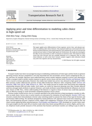
4. 76 C.-W. Yang, C.-C. Chang / Transportation Research Part E 47 (2011) 73–84
HSR cabin choice
scale factor
µ µ
R-Cabin U-Cabin R-Cabin U-Cabin
RP data SP data
Fig. 1. The estimation framework for combining RP and SP data.
strategy and cabin allocation do not match travelers’ demand very well. Therefore, we tried to identify the factors that
significantly influence travelers’ choice of R-cabin and U-cabin and find a cabin attribute strategy that could appreciably
affect cabin allocations. Thus, besides collecting RP data on cabin choice of HSR travelers, this paper adopts an SP technique
to find the important attributes that influence cabin choice.
3.2. Design of stated-preference
Previous studies indicate that fare class, time segment (peak/off-peak time), and advance reservation significantly influ-
ence choice of cabin/train class (Espino et al., 2008; Hensher, 2001; Proussaloglou and Koppelman, 1999). The current pricing
strategy in Taiwan’s HSR is based on both cabin class and time segment (e.g., weekday/weekend, peak/off-peak). To clarity
time segment effects in the existing pricing policies, we isolated time segment as an independent variable, representing its
influence by discount levels applicable to both cabin types. In order to evaluate the effect of advance purchase on the choice
of reserved-seat cabins, different levels of fare discount were designed to test travelers’ responses. Advance purchase dis-
count is designed only for R-cabin so its influence on cabin choice can be investigated. Thus, besides base fares for both cabin
types, SP scenarios involve three fare discounts: two time discounts, one for each cabin type, and an advance purchase dis-
count. To reflect the fare premium in corresponding to actual traveling distance, three discount levels were designed as per-
centage instead of absolute value of fare (Espino et al., 2008; Roman et al., 2007). This way is coincided with the practical
operating of Taiwan HSR.
In addition, since U-cabin cannot provide seat reservation, travelers may possibly have to remain standing through the
journey. Therefore, the probability of standing seat associated with U-cabin is factored into the SP scenario to represent
its disutility effect on cabin choice. This attribute can also be used to measure the monetary value of seat uncertainty.
For reasons mentioned above, the SP experiment involved three-level attributes that were used to design two alterna-
tives: R-cabin and U-cabin. The attributes are time segment discounts (R-cabin and U-cabin), advance purchase discount
(R-cabin), and standing seat probability (U-cabin). Because of cabin characteristics, the last two attributes are designed spe-
cifically for R-cabin and U-cabin, respectively. Since these attributes vary across time and between days, their corresponding
levels were designed according to time segments: weekday/weekend and peak/off-peak hours. The attribute levels in Table 1
were discussed with the HSR operators to determine reasonable ranges. The rules are that the weekday/off-peak time seg-
ment discount is higher than or equal to the weekend/peak-hour discount, and the weekend/peak-hour standing seat prob-
ability of U-cabin is higher than or equal to the weekday/off-peak probability. The earlier the ticket is purchased, the higher
would be the purchase discount. As a discount is provided for advance purchase, a fee of 10% of the fare is charged as the
trade-off for this attribute if the ticket is canceled (Espino et al., 2008; Proussaloglou and Koppelman, 1999).
Four designed attributes are provided: two time segment discounts for R-cabin and U-cabin, advance purchase discount,
and probability of standing seat. Thus, we have a full factorial design—81 combinations of four attributes each at three levels
(34). The principle of orthogonal fractional factorial design (L9(34)) is used to eliminate combinations of attributes and levels
(Espino et al., 2007; Hensher et al., 2008; Hess et al., 2007; Louviere et al., 2000; Park and Ha, 2006). A nine-profile was gen-
erated as the final SP scenario (S1–S9). Since our survey was carried out at HSR station, respondents would not have enough
time to answer the questionnaire. Hence, we randomly assigned the nine profiles to blocks of three, each of which consti-
tuted a version of the SP questionnaire (types A–C) (as Table 2). That means each respondent only have to answer three
SP scenarios and indicate his/her current RP choice regarding cabin class. The shorter questionnaire will help to raise the
willingness of respondents to participate our survey.
An example of an SP cabin scenario is presented in Table 3. It may be noted that the fee charge for cancelation of reserved
tickets is also illustrated in the SP scenario—a reminder to respondents.

5. C.-W. Yang, C.-C. Chang / Transportation Research Part E 47 (2011) 73–84 77
Table 1
Attributes and levels of cabin alternatives.
Levels of attributes Time segment discount (%) Advance purchase discount (R-cabin only) (%) Standing seat probability (U-cabin only)
Weekday
Peak R-cabin: 10/15/20 0 (departure day) 0.1
U-cabin: 20/25/ 30 10 (1 week ago) 0.2
20 (2 weeks ago) 0.3
Off-peak R-cabin: 20/25/30 0 (departure day) 0
U-cabin: 30/35/40 10 (1 week ago) 0.1
20 (2 weeks ago) 0.2
Weekend
Peak R-cabin: 0/5/10 0 (departure day) 0.2
U-cabin: 10/20/30 10 (1 week ago) 0.3
20 (2 weeks ago) 0.4
Off-peak R-cabin: 0/5/10 0 (departure day) 0
U-cabin: 10/20/30 10 (1 week ago) 0.1
20 (2 weeks ago) 0.2
Notes: (1) Weekdays are from Monday to Thursday; the weekend is Friday to Sunday.
(2) The weekday peak time is from 7 a.m. to 10 a.m. and 4 p.m. to 7 p.m., and weekend peak is from 4 p.m. to 9 p.m., Friday and Sunday. Off-peak refers to
the rest of the time.
Table 2
An example of orthogonal design for peak and weekday.
Scenario # Time segment discount (%) Standing seat probability (U-cabin) Advance purchase discount (R-cabin) (%) Type
R-cabin U-cabin
S1 10 (1) 20 (1) 0.1 (1) 0 (1) A
S2 10 (1) 25 (2) 0.2 (2) 10 (2) B
S3 10 (1) 30 (3) 0.3 (3) 20 (3) C
S4 15 (2) 20 (1) 0.2 (2) 20 (3) B
S5 15 (2) 25 (2) 0.3 (3) 0 (1) C
S6 15 (2) 30 (3) 0.1 (1) 10 (2) A
S7 20 (3) 20 (1) 0.3 (3) 10 (2) C
S8 20 (3) 25 (2) 0.1 (1) 20 (3) A
S9 20 (3) 30 (3) 0.2 (2) 0 (1) B
Table 3
An example of stated-preference experiments (S3).
Cabin class Time segment discount Advance purchase discount Standing seat probability
Reserved-seat (R-cabin) 10% 20% (2 week in advance) (10% fee charged if canceled) 0
Unreserved-seat (U-cabin) 30% No 0.3
Although this study adopt orthogonal experiments to design SP scenarios, we should recognize the fact that so-called D-
efficient design are able to produce more efficient data in the sense that more reliable parameter estimates can be achieved
with an equal or lower sample size (Bliemer and Rose, 2005; Rose and Bliemer, 2005, 2008). This efficient SC design has been
applied to MNL, NL, and ML model (Bliemer and Rose, 2010; Bliemer et al., 2009; Rose et al., 2008). On the future extension of
this study, the efficient of SP design could be involved in considering of data collecting method.
3.3. Sample survey and profile
A survey of travelers who journeyed more than 150 km was conducted at HSR station in October 2008. Each respondent
required to complete a self-administered questionnaire which was structured into three parts: RP cabin choice, SP scenarios,
and traveler characteristics. Respondents were sampled over weekdays and at weekends as well as at peak and off-peak
hours, so cabin choice behavior across various time segments could be captured. The full sample consisted of 330 respon-
dents. Each respondent represented one RP sample and three SP samples, in a questionnaire. The sample profile for both ca-
bin types is illustrated in Table 4.
Of the 330 respondents, male travelers accounted for 57%. Most of the respondents were in the age group of 30–49 years;
nearly 90% were between 18 and 49 years. Almost 60% of all respondents received a household income of NT$60,000–
NT$120,000 (US$1 = NT$32, 2010). The RP data, chosen for cabin class statistics, show that socioeconomic characteristics

6. 78 C.-W. Yang, C.-C. Chang / Transportation Research Part E 47 (2011) 73–84
Table 4
Sample characteristics for both cabins.
Characteristics Categories Cabin class
R-cabin U-cabin
Samples (%) Samples (%)
Gender Male 80 (52) 108 (61)
Female 74 (48) 68 (39)
Age 30 51 (33) 90 (51)
30–49 79 (51) 73 (41)
49 24 (16) 13 (8)
House income (NT$1000) 60 34 (22) 57 (32)
60–120 94 (61) 99 (57)
120 26 (17) 20 (11)
Fare expense Self-paid 110 (71) 151 (86)
Paid by others 44 (29) 25 (14)
Partner Single 63 (41) 95 (54)
Group 91 (59) 81 (46)
Day type Weekday 45 (29) 78 (44)
Weekend 109 (71) 98 (56)
When the trip is scheduled Occasional 4 (3) 31 (17)
In a week 104 (68) 122 (66)
Over a week 46 (29) 30 (17)
tend to favor males and younger age groups in the U-cabin and higher household income travelers in the R-cabin. With re-
gard to trip characteristics, 29% of R-cabin and 14% of U-cabin fares were paid by third parties. This is quite natural, because
travelers do not consider the cost of ticket and will choose more comfortable cabins where the fare is paid by others. Fur-
thermore, most R-cabin travelers tend to travel in groups (59%) and in the weekend (71%). Finally, the occasional traveler
favors the U-cabin (17%) rather than the R-cabin (3%), because the U-cabin class offers more flexible schedules.
According to RP data, cabin shares of R- and U-cabin are 47% and 53%, respectively. Further, 73% of R-cabin travelers
would choose the same cabin in both RP and SP experiments, the corresponding ratio for the U-cabin being 65%. These high
ratios indicate a strong inertia effect in cabin choice behavior. Furthermore, the ratio of travelers who switch from U-cabin
(RP) to R-cabin (SP) is 35% higher than the other way round (27%). This means U-cabin travelers are more likely to switch
their cabin preference as a result of the influence of SP attributes.
4. Results
Prior to construct a cabin choice model with combining RP and SP data, we first used RP data to test the most fitting model
specification. This way could be more efficiency in identifying effective variables and speeding model convergence while
combing two different data sources. Then the proposed specification in effective variables and model structure is used to
construct a cabin choice model with RP and SP data. Finally, a scenario analysis is undertaken to interpret the implications.
4.1. Model specifications
We first used MNL model to identify those effective variables and then estimated two alternative ML formulations to
determine the most fitting model specification. The variables used in the utility function of MNL model can be classified into
four types and their meaning and specification are explained in the following paragraphs:
1. Constants and scale factor: For the U-cabin, an alternative specified constant (ASC), one each for the RP and SP data, and an
inertia constant to capture the habitual effect within SP data were assigned. The inertia variable in SP utility equals to 1 if
U-cabin was chosen in RP data and otherwise equals to 0. In addition a scale factor is used to represent the ratio of vari-
ances of error terms between RP and SP data.
2. Cabin attributes: Fare represents the ticket cost. It corresponds to travel distance and is specified as a common variable for
both cabin classes. In RP, the fare is self-reported by respondents, while in SP the fare is adjusted by all available dis-
counts, including time segment and advance purchase discounts. To avoid zero values, the time discount variable was
specified as a ratio of adjusted fares (1 À time discount)—R-cabin’s relative to U-cabin’s. This ratio is used to measure
the time segment effect on cabin choice. While considering the effect of seat availability, we should remember that stand-
ing seat probability is specific to the U-cabin.
3. Trip characteristics: A dummy variable of fare expense was included to examine the influence of third-party-paid trips on
cabin choice. Moreover, two dummy variables, one for occasional trips and another for the single traveler, were specified

7. C.-W. Yang, C.-C. Chang / Transportation Research Part E 47 (2011) 73–84 79
to reflect the flexibility of schedule selection and seat availability in the U-cabin. Finally, a dummy weekday variable was
specified for the U-cabin to reveal the difference in cabin preference between weekdays and weekends.
4. Socioeconomic background: Household income of R-cabin travelers was studied to examine if higher-income travelers
would prefer higher-fare classes for its comfortable cabin. In addition, a dummy variable was specified for gender to
explore how male and female travelers’ cabin preferences differ.
The results of two MNL models were summarized in first two columns of Table 5 (MNL1 and MNL2). All of the coefficients
have the expected sign and are statistically significant except for fare. To consist with the microeconomic principles of dis-
crete model choice model, we first adopt the specification of dividing fare by ln(income) to accommodate income effect in all
indirect utility expression (Jara-Díaz and Farah, 1987; Jara-Díaz and Videla, 1989; Train and McFadden, 1978) (see MNL1
model). However, this way was not found expected sign and statistically significant. But interestingly, if the income was
specified solely to R-cabin as alternative specified variable (Greene and Hensher, 2007; Hensher, 2008), its coefficient and
model fitness will be improving significantly (see MNL2 model). Since data limitation in collecting qualitative cabin attri-
butes, the income is used to represent as a proxy of comfort tendency.
Furthermore, we used two ML models (ECL and RCL) to consider the heterogeneity across alternatives and individuals.
Their estimating results are listed as the third and fourth columns of Table 5. Two error components of R-cabin and U-cabin
in ECL model were not statistically significant. Also, the likelihood ratio test between MNL2 and ECL ðÀ2½ðÀ195:77ÞÀ
ðÀ194:92ÞŠ ¼ 1:7 v2 2;0:05 ¼ 5:99Þ indicated that ECL model is not statistically significant than MNL2 model. The result is con-
sistence of our preliminary investigations on those demographic variables did not find additional significant interactions
with cabin attributes.
Then we specified fare variable as random coefficient with normal distribution. The standard deviation of fare coefficient
is 0.014 and not quite significant (t-value = 1.4). The likelihood ratio statistic for RCL versus MNL2 is 2.94 with comparing to
critical value (v21;0:05 ¼ 3:84), which reveals RCL model is not statistically significant than MNL2 model. In our empirical
study, two heterogeneous ML models are not significant than MNL model. That revealed that those segments by trip and
socioeconomic characteristics with specifying as additive dummy variables had explained out most part of heterogeneity
across alternatives and individuals. Hence, the specification of MNL2 model is used to construct the cabin choice model with
joint RP and SP data.
4.2. Cabin choice model with joint RP/SP data
Before using RP and SP data to modeling cabin choice behavior, we should first investigate the correlation between three
SP scenarios responded by the same traveler. This paper assumes that the correlation among responses could be distin-
guished into two parts: one is between RP and SP data and the other is among SP responses of the same person. The former
could be conducted with the inertia variable to reflect RP influence in SP model. As regards to the latter, although the error
Table 5
The estimation results of cabin choice model-RP data.
MNL1 MNL2 ECL RCL
Coefficient t-Value Coefficient t-Value Coefficient t-Value Coefficient t-Value
Constant
U-cabin alternative À0.794 À3.1 À0.061 À0.2 0.025 0.1 0.198 0.3
Cabin attributes
Fare (NT$1000) À0.863 À0.9 À0.921 À1.0 À0.369 À0.1
Standard deviation of fare 0.014 1.4
Fare/ln(income) 2.060 0.1
Trip characteristics
Others-paid trip (R)* 1.420 4.5 1.386 4.3 1.491 3.5 1.991 3.0
Occasional trip (U) 2.015 3.7 2.176 4.3 2.330 3.1 3.071 2.6
Weekday (U) 1.012 3.7 1.133 4.1 1.199 3.6 1.451 3.0
Single traveler (U) 0.601 2.5 0.667 2.7 0.712 2.5 0.969 2.3
Socioeconomic background
Income (R) 1.154 2.9 1.161 2.5 1.523 2.2
Man (U) 0.507 2.1 0.618 2.4 0.649 2.3 0.808 2.1
Error component
Standard deviation of R-cabin 0.050 0.1
Standard deviation of U-cabin 0.519 0.8
Samples 330 330 330 330
LL(0) À228.74 À228.74 À228.74 À228.74
LL(b) À200.35 À195.77 À194.92 À194.29
q2 0.124 0.144 0.148 0.151

8. 80 C.-W. Yang, C.-C. Chang / Transportation Research Part E 47 (2011) 73–84
generation process for a collection of SP choices in a controlled experiment might be expect to be the same, it is likely to be
different variation across SP scenarios. Hence, we used panel ECL model to investigate the correlation between three SP
choices (Brownstone et al., 2000). In the panel data or repeated choices, the error term gi of Eq. (4) is specified as a random
effect that induces correlation across observations of the same individual. The results of ECL model with SP data are listed as
first column of Table 6 (see ECL-SP model). The error components relating two alternatives are not statistically significant.
Hence, we assumed the error terms are independent across SP choices made by the same individual (Brownstone et al., 2000;
Hess, 2008; Mabit et al., 2008; Train, 2003).
Based on prior investigations on model specification and correlations across observations made by the same individual,
we adopted the specification of MNL2 model to construct a cabin choice model with combining RP and SP data. The estima-
tion results are shown in second column of Table 6 (see MNL-JP model). Likelihood ratio test results indicate that the null
hypothesis of all parameters is zero and can be rejected at a 5% level of significance. This means the proposed model has
a good fit. All coefficients of cabin attributes are negative and significant, except that of standing seat probability. The fare
variable incorporates the effects of all types of discounts, including cabin class, time segment, and advance purchase. The
time discount variable captures the effect of both classes’ time segment discount on cabin choice. Although the fare variable
includes the effect of time segment discount, we designed the ratio as a solo variable to investigate if the time discount strat-
egy influences cabin choice significantly. Its coefficient is fairly significant and has a negative effect. This means travelers will
prefer the R-cabin if the time discounts of both cabins are more or less same. This result indicates that although the model
considers ticket fare, the relative difference between time discounts for both cabins plays an important role. In other words,
besides the monetary effect of fare, the psychology effect of time segment discount influences cabin choice considerably.
The coefficient of standing seat probability for the U-cabin is less significant (though significance level is more than 90%).
This may be due to the fact that the load factor of HSR has not reached the saturation level and, therefore, travelers could not
consider the attribute more seriously. However, the negative coefficient indicates that the penalty of uncertainty about seat
availability plays an adversarial role in influencing a choice in favor of the U-cabin. In addition, although the attribute of ad-
vance purchase discount could not be specified as a significant variable, its influence has been considered through the fare
variable.
As regards the trip and socioeconomic characteristics, we had specified those variables as interaction with cabin attri-
butes in prior investigation. For example, the interaction of others-paid trip with fare (LL(b) = À761.049) and single traveler
with standing seat probability (LL(b) = À763.893) are not statistically significant than the specification of additive dummy
variable on model fitness or corresponding t-value. Hence, we specified trip and socioeconomic characteristics as alternative
specified variable to reveal the differences between trip and socioeconomic segments. As the results, the variable represent-
ing fares paid by others has a statistically significant influence on the choice of R-cabin. The positive coefficient implies that
Table 6
The estimation results of cabin choice model-SP data and Joint data.
Variables ECL-SP MNL-JP
Coefficient t-Value Coefficient t-Value
Constant
U-cabin (RP) 0.008 0.01
U-cabin (SP)* À8.148 À5.0 À13.31 À3.4
Inertia (U-cabin) (SP)* 2.383 6.5 3.131 3.4
Scale factor 0.447 4.0
Cabin attributes
Fare (NT$1000) À2.877 À2.4 À1.659 À2.1
Time discount ratio (R-cabin)*(SP)* À6.434 À4.9 À9.917 À3.3
Standing seat probability (U-cabin)(SP)* À4.345 À3.9 À2.033 À1.3
Trip characteristics
Others-paid trip (R-cabin) 0.656 4.2 1.190 4.0
Occasional trip (U-cabin) 2.350 0.6 2.636 4.6
Weekday (U-cabin) 0.194 0.5 0.883 3.5
Single traveler (U-cabin) 0.373 1.2 0.618 2.9
Socioeconomic background
Income (R-cabin) 0.867 1.7 0.117 3.2
Man (U-cabin) 0.134 0.4 0.498 2.4
Error component
Std (R-cabin) 0.964 0.2
Std (U-cabin) 1.872 0.7
Samples 990 1320
LL(0) À686.849 À914.954
LL(b) À513.195 À761.152
q2 0.253 0.168
*
Those variables are only specified to SP utility.

9. C.-W. Yang, C.-C. Chang / Transportation Research Part E 47 (2011) 73–84 81
these travelers prefer a higher-fare alternative since they do not usually consider the ticket fare while deciding on a cabin
class. The occasional trip coefficient has a significant positive influence on a choice in favor of the U-cabin. Similar is the case
with the single traveler. This may be due to the fact that the U-cabin offers more flexibility in schedule selection. The positive
coefficient of the weekday trip indicates that weekday travelers prefer the U-cabin.
In terms of socioeconomic characteristics, the specification of income variable had been addressed as well as RP model.
The household/personal income are not significant neither dividing it into fare nor segmenting it as an interaction with fare,
but as an R-cabin specified variable. The income variable supposes to represent as a proxy of comfort tendency. The positive
coefficient means the travelers with high household income prefer the higher-fare R-cabin class for more comfort. Further,
male travelers are more likely to choose the U-cabin than are female travelers. The main reason is that female travelers are
more concerned about the privacy of cabin environment. They would prefer a cabin with seat reservation facility. Finally, the
inertia variable of U-cabin has a statistically significant positive influence on cabin choice. Results indicate that the inertia
effect plays an important role in the combined RP and SP data. The scale factor (0.447) shows that SP data variance is 2.2
times the variance in RP data. In addition, ASC represent the shares of both cabins, it should be specified respective to RP
and SP to reveal the share differences across data sets (Brownstone et al., 2000; Ortúzar and Iacobelli, 1998). Hence, the
ASC of U-cabin for RP data is still reserved in MNL-JP model.
4.3. Discussion and implication
A scenario analysis is proposed to examine the sensitivity of cabin shares to changes in cabin attributes. The main focus is
on the discount attribute for time segment. Those variables of MNL-JP model in Table 6 were used to process scenario anal-
ysis while the inertia variable for SP is not used in forecasting (Ortúzar and Iacobelli, 1998). The scenarios (named Regular,
Blue, and Orange trains) are designed according to current pricing rules of Taiwan HSR to examine the rationality of the pres-
ent cabin allocation system. The following scenarios consider the extra discount based on different time segments apart from
the nearly 15% fare difference between both cabins. In the Regular train scenario, with 15% off in U-cabin fares, 64% of the
travelers prefer the U-cabin. Of a total of eleven standard cabins, seven (0.64 Ã 11 = 7.04) are required for U-cabin allocation.
On the same principle, five U-cabin and eight R-cabin for Blue and Orange train, respectively, would be ideally required
to satisfy the demand of both cabins (see Table 7). These results suggest that R- and U-cabin allocations should be done
Table 7
Scenario analysis for time segments.
Time segment Fare discount Predicted share (%) Number of cabins
R-cabin U-cabin R-cabin U-cabin
Regular train
R-cabin – 36 64 4 7
U-cabin 15% off
Blue train
R-cabin 15% off 52 48 6 5
U-cabin 15% off
Orange train
R-cabin 35% off 72 28 8 3
U-cabin 15% off
Table 8
Cabin share changes in segments based on trip characteristics.
Types of trip characteristics Predicted share (%) Changes of share (%)
R-cabin U-cabin R-cabin U-cabin
Fare source
Self-paid 49 51 +13 À13
Paid by others 62 38
Day type
Weekday 46 54 +9 À9
Weekend 55 45
Traveling partner
Single 48 52 +7 À7
Group 55 45
Scheduled type
Occasional trip 45 55 +10 À10
Planned trip 55 45

10. 82 C.-W. Yang, C.-C. Chang / Transportation Research Part E 47 (2011) 73–84
according to the scenario presented here. However, existing cabin allocations in Taiwan HSR are not flexible and even involve
cancelation of U-cabin services on certain days. Thus, capacities of different cabin types are not adequate to match demand
in full. This leads to unoccupied or overcrowded cabins.
To evaluate the impact of trip characteristics on cabin choice, we calculated the predicted cabin shares based on the seg-
ments of trip characteristics. Results are summarized in Table 8. Third-party-paid trips are 13% more than self-paid trips in
the R-cabin class. Regarding day type, more weekday (9%) than weekend travelers choose U-cabin class. The same trend ap-
pears in traveling-partner and scheduled types. More single (7%) than group travelers choose U-cabin class, as do occasional
travelers—10% more than the planned type. These results of cabin share changes can help HSR operators frame more effec-
tive cabin strategies based on trip characteristics of each segment.
Finally, according to the foregoing empirical results, travelers are willing to pay NT$123 ð½ðÀ2:033=100Þ=
ðÀ1:659=1000ÞŠ à 10Þ for a 10% improvement in the seating probability of a U-cabin. For example, the difference between
the two cabin class fares is about 15% of an R-cabin ticket (NT$1490) for the longest trip in Taiwan HSR, which is equal to the
monetary value of a 20% improvement in the seating probability of a U-cabin. The equation is as follows:
ð1490 Â 15%Þ=123 ¼ 2 ( 20% improvement in seating probability
) ð8Þ
This means that if the probability of standing seat in the U-cabin increases by 20%, travelers will tend to choose the R-
cabin. Therefore, HSR operators should remember the critical limitations to cabin allocation arrangements.
5. Conclusions
A few studies on intramodal competition between service classes consider cabin class as a single alternative to model
choice behavior. The paper identifies cabin choice preferences with the MNL model and examines cabin attributes designed
by the stated-preference method. The advantages of combining RP and SP data were presented. These related to the accuracy
of travelers’ responses and trade-off of cabin attributes. The proposed model was validated using cabin choice data collected
from HSR travelers, with cabins classified as reserved and unreserved.
The primary contribution of the paper is applying price differentiation based on time, service class, and advanced pur-
chase to modeling the cabin choice behavior of HSR while previous literatures were not concerned with all of them simul-
taneously (Hensher, 1997, 2001; Ortúzar and Simonetti, 2008; Park and Ha, 2006). Furthermore, this study also has
estimated the monetary value of standing seat probability and to evaluate the effect of seat uncertainty. This issue is such
important on traveling choice behavior but rarely addressed in literatures. An another practical contribution is the scenario
analysis can help operators to make the most appropriate strategy of cabin allocation in corresponding to time segment and
trip characteristics.
The results indicated that cabin attributes of fare, time discount ratio, and standing seat probability influence cabin
choice. In common with many previous studies (Espino et al., 2008; Hensher, 2001; Proussaloglou and Koppelman, 1999),
fare level is an important and easy-measured quantitative factor when travelers facing to choose a preferred cabin class
within the same mode. Another interesting finding is the significance of the time discount ratio. The monetary value of seat
uncertainty can be calculated from the ratio of the coefficient of standing seat probability to that of fare. Results reveal that
the upper limit of standing seat probability for U-cabin is 20%. Above this level, travelers would be willing to pay an extra
15% to upgrade to R-cabin.
This paper designed an attribute to examine the effect of discriminatory pricing based on time segment. Rarely have cabin
choice modeling studies investigated the influence of time segment, previously. The relevant coefficient evidenced that time
segment pricing strategy explicitly affects travelers’ preferences. The results of scenario analysis also show that time seg-
ment strategies lead to obvious cabin share changes. Therefore, the allocation of both cabin types should correspond to time
segment demand.
Within segments based on trip characteristics, cabin shares change substantially and differently. Travelers whose fares
are paid by others prefer the reserved-seat cabin service. Therefore, marketing strategy for R-cabin should focus mainly
on business travelers. The HSR operator can effectively maintain loyal relationships with commercial companies by ticketing
premium contracts. Furthermore, the group premium strategy can be used to raise the R-cabin loading factor. In other words,
the positioning of U-cabin should target the weekday and occasional trip segments. The common feature of these segments
is the issue of flexibility of schedules and mobility. As U-cabin does not need to be assigned train schedules and seat num-
bers, introduction of payment mechanisms such as the stored value card, for example, the Octopus Card in Hong Kong, can
speed up the ticketing process and platform access.
In spite of these remarkable findings, a number of issues remain to be considered in future research. The major purpose of
this study is only to focus on intra-competition for HSR cabins. However, cabin choice behavior can also influence intermodal
competition. Hence, future research should combine mode choice and cabin choice, simultaneously, to investigate the effects
of cabin strategy on intermodal and intramodal competition. Besides, this study considers only two types of standard cabins
but ignores the business class cabin. The role of the business cabin class in the context of growth of HSR demand is an impor-
tant area for further investigations.
Regarding to the reviewing of research methodology, this study assumes the unobserved error terms are independent
across RP and SP responses made by the same traveler. However, the limitation may require further amendment by alter-

11. C.-W. Yang, C.-C. Chang / Transportation Research Part E 47 (2011) 73–84 83
native models, e.g., panel error component mixed logit model (Hensher, 2008; Hensher et al., 2008; Hess and Rose, 2009). In
addition, an alternative method relative to orthogonal experiment for SP design, so-called D-efficiency, has been proved in
producing more efficient and reliable parameter estimation for discrete choice models (Bliemer and Rose, 2010; Bliemer
et al., 2009; Rose et al., 2008). The future study could involve the consideration with the efficient SP design.
Acknowledgments
The authors gratefully acknowledges the helpful comments of Professor Wayne K. Talley and the anonymous reviewers
who provided valuable input and comments that have contributed to improve the content of this paper. The authors also
thank Shao-Feng Yuen for his assistance on data collection and preliminary analysis. This research is supported in part by
National Science Council of the Republic of China in Taiwan under Grants NSC 98-2410-H-025-008-SSS.
References
Ben-Akiva, M., Lerman, S., 1985. Discrete Choice Analysis: Theory and Application to Travel Demand. MIT Press, Cambridge, Mass.
Ben-Akiva, M., Morikawa, T., 1990. Estimation of travel demand models from multiple data sources. In: 11th International Symposium on Transportation
and Traffic Theory, Yokohama.
Ben-Akiva, M., Morikawa, T., 2002. Comparing ridership attraction of rail and bus. Transport Policy 9, 107–116.
Bhat, C.R., 1998. Accommodating variations in responsiveness to level-of-service measures in travel mode choice modeling. Transportation Research Part A
32, 495–507.
Bliemer, M.C.J., Rose, J.M., 2005. Efficiency and Sample Size Requirements for Stated Choice Studies. Working Paper: ITLS-WP-05-08.
Bliemer, M.C.J., Rose, J.M., 2010. Construction of experimental designs for mixed logit models allowing for correlation across choice observations.
Transportation Research Part B 44, 720–734.
Bliemer, M.C.J., Rose, J.M., Hensher, D.A., 2009. Efficient stated choice experiments for estimating nested logit models. Transportation Research Part B 43,
19–35.
Bradley, M., Daly, A.J., 1997. Estimation of logit choice models using mixed stated preference and revealed preference information. In: Stopher, P., Lee-
Gosselin, M. (Eds.), Understanding Travel Behaviour in an Eraof Change. Pergamon, Oxford.
Brownstone, D., Train, K., 1999. Forecasting new product penetration with flexible substitution patterns. Journal of Econometrics 89 (1), 109–129.
Brownstone, D., Bunch, D.S., Train, K., 2000. Joint mixed logit models of state and revealed preferences for alternative-fuel vehicles. Transportation Research
Part B 34, 315–338.
Espino, R., Ortúzar, J.de D., Roman, C., 2007. Understanding suburban travel demand: flexible modeling with revealed and stated choice data. Transportation
Research Part A 41, 899–912.
Espino, R., Martin, J.C., Roman, C., 2008. Analyzing the effect of preference heterogeneity on willingness to pay for improving service quality in an airline
choice context. Transportation Research Part E 44, 593–606.
Greene, W.H., Hensher, D.A., 2007. Mixed logit and heteroscedastic control for random coefficients and error components. Transportation Research Part E
43, 610–623.
Hensher, D.A., 1997. A practical approach to identifying the market potential for high speed rail: a case study in the Sydney–Canberra corridor.
Transportation Research Part A 31, 431–446.
Hensher, D.A., 1998. Establishing a fare elasticity regime for urban passenger transport. Journal of Transport Economics and Policy 32 (2), 221–246.
Hensher, D.A., 2001. The sensitivity of the valuation of travel time savings to the specification of unobserved effects. Transportation Research Part E 37, 129–
142.
Hensher, D.A., 2008. Empirical approaches to combining revealed and stated preference data: some recent developments with reference to urban mode
choice. Research in Transportation Economics 23, 23–29.
Hensher, D.A., Raimond, T., 1995. Evaluation of Fare Elasticities for the Sydney Region. Report Pre-pared by the Institute of Transport Studies for the NSW
Government Pricing Tribunal, Sydney.
Hensher, D.A., Rose, J.M., Greene, W.H., 2008. Combining RP and SP data: biased in using the nested logit ‘trick’-constants with flexible mixed logit
incorporating panel and scale effects. Journal of Transport Geography 16, 126–133.
Hess, S., 2008. Treatment of reference alternatives in stated choice surveys for air travel choice behaviour. Journal of Air Transport Management 14, 275–
279.
Hess, S., Rose, J.M., 2009. Allowing for intra-respondent variations in coefficients estimated on repeated choice data. Transportation Research Part B 43, 708–
719.
Hess, S., Bierlaire, M., Polak, J.W., 2005. Estimation of value of travel time savings using mixed logit models. Transportation Research Part A 39, 221–236.
Hess, S., Adler, T., Polak, J.W., 2007. Modelling airport and airline choice behavior with the use of sated preference survey data. Transportation Research Part
E 43, 221–233.
Jara-Díaz, S., Farah, M., 1987. Transport demand and user’s benefits with fixed income: the goods/leisure trade-off revisited. Transportation Research Part B
21, 165–170.
Jara-Díaz, S., Videla, J., 1989. Detection of income effect in mode choice: theory and application. Transportation Research Part B 23, 394–400.
Louviere, J., Hensher, D., Swait, J., 2000. Stated Choice Methods: Analysis and Applications. Cambridge University Press, New York.
Mabit, S., Hess, S., Caussade, S., 2008. Correlation and Willingness-to-Pay Indicators in Transport Demand Modelling. Paper Presented at the 87th Annual
Meeting of the Transportation Research Board, Washington, DC.
McFadden, D., 1973. Conditional logit analysis of qualitative choice behavior. In: Frontiers in Econometrics. Academic Press, New York.
McFadden, D., 1978. Modeling the choice of residential location. In: Karlquist, A., Lundquist, L., Snickars, F., Weibull, J.W. (Eds.), Spatial Interaction Theory
and Planning Models. North-Holland, Amsterdam, The Netherlands.
McFadden, D., Train, K., 2000. Mixed MNL models for discrete response. Journal of Applied Econometrics 15, 447–470.
Nuzzolo, A., Crisalli, U., Gangemi, F., 2000. A behavioural choice model for the evaluation of railway supply and pricing policies. Transportation Research Part
A 34, 395–404.
Ortúzar, J.de D., Iacobelli, A., 1998. Mixed modelling of interurban trips by coach and train. Transportation Research Part A 32, 345–357.
Ortúzar, J.de D., Simonetti, C., 2008. Modeling the demand for medium-distance air travel with the mixed data estimation method. Journal of Air Transport
Management 14, 297–303.
Ortúzar, J.de D., Willumsen, L.G., 2001. Modelling Transport, third ed. John Wiley Sons, Chichester.
Park, Y., Ha, H.K., 2006. Analysis of the impact of high-speed railroad service on air transport demand. Transportation Research Part E 42, 95–104.
Proussaloglou, K., Koppelman, F.S., 1999. The choice of air carrier, flight, and fare class. Journal of Air Transport Management 5, 193–201.
Revelt, D., Train, K., 1998. Mixed logit with repeated choices: households’ choices of appliance efficiency level. Review of Economics and Statistics 80, 647–
657.

12. 84 C.-W. Yang, C.-C. Chang / Transportation Research Part E 47 (2011) 73–84
Roman, C., Espino, R., Martin, J.C., 2007. Competition of high-speed train with air transport: the case of Madrid–Barcelona. Journal of Air Transport
Management 13, 277–284.
Rose, J.M., Bliemer, M.C., 2005. Sample Optimality in the Design of Stated Choice Experiments, Working Paper: ITLS-WP-05-13.
Rose, J.M., Bliemer, M.C.J., 2008. Constructing Efficient Stated Choice Experimental Designs. Paper Presented at the TRB Workshop: Observing Complex
Choice Behavior with Stated-preference Experiments: Innovations in Design, Washington, DC.
Rose, J.M., Hensher, D.A., Greene, W.H., 2005. Recovering costs through price and service differentiation: accounting for exogenous information on attribute
processing strategies in airline choice. Journal of Air Transport Management 11, 400–407.
Rose, J.M., Bliemer, M.C.J., Hensher, D.A., Collins, A.T., 2008. Designing efficient stated choice experiments in the presence of reference alternatives.
Transportation Research Part B 42, 395–406.
Train, K., 1998. Recreation demand models with taste variation over people. Land Economics 74, 230–239.
Train, K., 2003. Discrete Choice Methods with Simulation. Cambridge University Press, New York.
Train, K., McFadden, D., 1978. The goods/leisure tradeoff and disaggregate work trip mode choice models. Transportation Research 12, 349–353.
Wardman, M., Toner, J., 2003. Econometric modeling of competition between train ticket types. In: Proceedings of the European Transport Conference,
London, UK, pp. 8–10.
Wen, C.H., Lai, S.C., 2010. Latent class models of international air carrier choice. Transportation Research Part E 46, 211–221.