1) Derivatives relate the rates of change of position, velocity, and acceleration. Velocity is the derivative of position and measures rate of change of displacement. Acceleration is the derivative of velocity and measures the rate of change of velocity. 2) The Mean Value Theorem states that for a continuous function over an interval, there exists at least one point where the slope of the tangent line equals the slope of the secant line between the endpoints. 3) A function's derivatives provide information about the behavior of the original function. The first derivative relates to slope and critical points where the function is increasing/decreasing. The second derivative indicates points of inflection where the concavity changes.

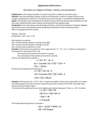
1. Application of Derivatives
Derivative as it relates to Position, Velocity, and Acceleration
Displacement is the change in position of a point or particle in relation to a previous point.
Velocity is how fast something is going, as well as in the direction in which it is going. Velocity is the
change in displacement, and thus is an instantaneous rate of change, or a derivative of displacement.
Speed is the absolute value of displacement. Speed increases when the velocity and acceleration are the
same sign. Speed decreases when velocity and acceleration have opposite signs.
Acceleration is the instantaneous rate of change of velocity, and thus the derivative of velocity. Negative
acceleration means a decreasing velocity and positive acceleration means increasing velocity.
With x as displacement and t as time:
Velocity = V(t)=x’(t)
Acceleration = a(t) = v’(t) = x’’(t)
With relation to a particle,
v(t) > 0 means that the particle is moving to the right
v(t) < 0 means that the particle is moving to the left
v(t) = 0 means that the particle is at rest.
Example 1: The position of a particle on a line is given by s(t) = t3 − 3 t2 − 6 t + 5, where t is measured in
seconds and s is measured in feet. Find
The velocity of the particle at the end of 2 seconds.
The acceleration of the particle at the end of 2 seconds.
Part (a): The velocity of the particle is
Part (b): The acceleration of the particle is
Example 2: The formula s(t) = −4.9 t2 + 49 t + 15 gives the height in meters of an object after it is thrown
vertically upward from a point 15 meters above the ground at a velocity of 49 m/sec. How high above
the ground will the object reach?
The velocity of the object will be zero at its highest point above the ground. That is, v = s′(t) = 0, where
The height above the ground at 5 seconds is

2. Mean Value Theorem
The mean value theorem basically states that for a smooth (differentiable) and continuous function
from [a,b], there exists a point, c, or points that have the same slope as the line connecting the
endpoints.
Essentially:
Example:
In checking to see where such a point is, one should first check that the function is continuous and
differentiable to verify that such a point could actually exist.
Ex. Does the following function meet the requirements of the Mean Value Theorem? If so find the value
c such that
1. Function Value:
Interval:
[-2, 7]
Steps:
Solve the equation for Y using the X values provided. Such yields the Y values 19 and 10,
respectively. Plugging into the slope equation yields an m of 1. According to the theorem, there
is at least one other point on this graph where m=1.
Differentiating the equation, one is left with:
f’(x) = 2x-6
In line with the theorem, substituting our representative variable of c with x and making this
equal to the slope we found, then:
2c – 6 = (f(7)-f(-2))/(7+2) = -1
And solving for x:
2c – 6 = -1
c = 5/2
At point c on the original graph, the slope is equal to that of the two endpoints given.
Plugging c into our original equation yields the y value at which this occurs, -5.75.

3. Connecting f, f’ and f’’
A wealth of information about a function can be found through its derivatives and double
derivatives. This relates to the initial topic covered regarding displacement, velocity and acceleration.
To summarize (Function used in example is included):
f(x) = The function at x = x3 – 4x2 + 5
f’(x)= The rate of change at x, namely, the slope at x = 3x2 – 8x
f’’(x) = The concavity of a function at x = 6x – 8
Taking advantage of such requires the finding of “critical points” on the graphs, points where behavior
of the graph changes.
To find critical points, set the derived equation equal to 0 and solve for x.
With regard to f’(x), these x values show where the slope of the original equation is zero. This could
mean the existence of a local maximum, minimum or just a temporary flattening out of the graph. To
determine what, plot these values on a number line.
Using the function from earlier, we set the derivative equal to 0 and find that
X = 0, 8/3
Considering that f’(x) tells us the slope at any point of the line f(x), The graph of f’(x) being zero at these
points must mean that at these points, the slope of the original graph is 0. As mentioned earlier, we
must use a “sign line” to find out what is happening.
With regards to f’(x):
When f’(x) > 0, f(x) is increasing.
Similarly,
When f’(x) < 0, f’(x) is decreasing
Using this, and plugging in a value lass than 0, between 0 and 8/3, and a value above 8/3, will give us the
behavior of the original graph.
f’(-1) = 11 (Positive!) Plugging this into our sign line, we get:
f’(1) = -5 (Negative!)
f’(3) = 3 (Positive!)
Concerning the original graph, this tells us that:
 from (-∞,0) The function is increasing,
 (0,8/3) The function is decreasing and
 from (8/3,∞)the function is once again increasing.
From this, we can surmise that at 0 there is a relative maximum (as the graph goes from going up to
going down at this point), and at 8/3 there is a relative minimum (as the graph changes from going up to
going down at this point).
...
f’’(x) is the second derivative of the original function. Using it we can determine the “concavity of the
original function.

4. The below picture demonstrates concavity:
Steps to find concavity are similar to those to determine where a graph increases and decreases.
Set the second derivative equal to 0 and solve for x. This will give us inflection points, places where the
graph changes concavity.
Using the Function from before,
f”(x) = 6x-8
Thusly,
x = 8/6 = 4/3
4/3 is a critical point, or more specifically,
a point of inflection.
We then use this value to make a sign line:
Plugging in values less than 4/3 and more than 4/3 we get:
f”(0) = -8 (Negative!) Putting this into our sign line we see that:
f”(2) = 4 (Positive!)
Where f”(x) > 0, f(x) is concave up
and
Where f”(x) < 0, f(x) is concave down
Essentially, The graph of f(x) is concave down from -∞ to 4/3 and concave up from 4/3 to ∞.
The above conclusions are verified by a look at the graph of x3 – 4x2 + 5

5. Related Rates
In dealing with equations that involve two or more variables that are differentiable functions of time t,
they can be differentiated to find an equation that relates the rates of change of these several variables.
By Implicit differentiation unknown related rates and such can be found.
Example 1: Air is being pumped into a spherical balloon such that its radius increases at a rate of .75
in/min. Find the rate of change of its volume when the radius is 5 inches.
The volume (V) of a sphere with radius r is
Differentiating with respect to t, you find that
The rate of change of the radius dr/dt = .75 in/min because the radius is increasing with respect to time.
At r = 5 inches, you find that
thus, the volume is increasing at a rate of 75π cu in/min when the radius has a length of 5 inches.
Example 2: A car is traveling north toward an intersection at a rate of 60 mph while a truck is traveling
east away from the intersection at a rate of 50 mph. Find the rate of change of the distance between the
car and truck when the car is 3 miles south of the intersection and the truck is 4 miles east of the
intersection.
Let x = distance traveled by the truck
y = distance traveled by the car
z = distance between the car and truck
The distances are related by the Pythagorean Theorem: x2 + y2 = z2 (Figure 1 )
The rate of change of the truck is dx/dt = 50 mph because it is traveling away from the intersection,
while the rate of change of the car is dy/dt = −60 mph because it is traveling toward the intersection.
Differentiating with respect to time, you find that

6. hence, the distance between the car and the truck is increasing at a rate of 4 mph at the time in
question.
Example 3: Water is being poured into a conical reservoir at the rate of pi cubic feet per second.
The reservoir has a radius of 6 feet across the top and a height of 12 feet. At what rate is the
depth of the water increasing when the depth is 6 feet?
Solution: h = depth of the water in the reservoir
r = radius of the water in the reservoir
The volume of the water in the reservoir (V) is given by

7. Application of Integrals
Displacement vs. Total Distance Traveled
Displacement = rate of change x time
As such, an equation showing the rate of change with respect to time can be integrated to find the area
under the graph – the displacement.
Displacement is a change in position relative to the starting point. Displacement takes into account
negative shifts in position and is essentially the net movement of any changes in position.
Example: Suppose the initial position of a particle is s(0) = 9. What is the particle’s position at t = 1, 5?
The equation of the movement of the particle is:
Integrate to find displacement after
One second:
After 5 seconds:
The new position after 1 second is = initial position + the displacement = 16/3
The new position after 5 seconds is = initial position + the displacement = 44
Distance travelled is similar to displacement, albeit distance does not take negative position changes
into account. Any position change is added positively to the total distance. To do so, one can use the
same integrand used for displacement, but taking all positive values, or:
Total Distance Travelled =
Integrating this on our calculator we arrive at the total distance travelled from 0, 5 as
This is total distance travelled with, while Displacement is but The net distance travelled.
Area Between Curves
The area between two curves can be found simply by subtracting the smaller area from the larger over a
given range, or

8. Such manipulation would allow for one to do problems involving two curves occurring simultaneously.
An example would be a curve showing the rate of people leaving a room plotted on the same graph as a
curve sowing the rate of people entering. The area between these two curves would represent the
number of people actually in the room at a given time.
Not all curves are as simple as the one above. At times, the curves may switch places, as in below. When
such happens, the integrand must be split into, the new integrand taking into account the switching of
roles between the two curves and starting at the intersection point (in this case, c):
Even more complications arise when a region is bounded by one curve for part of it as shown below.
Simply splitting it up into pieces as above can work, provided one takes into account a situation like
f(x)’s on the right of the graph, however, other methods are available. One could solve the integrals in
relation to the y axis as opposed to the x.
Examples of the three situations provided can be found on the next 2 pages.

11. Volume of a Solid of Revolution
Taking an equation and rotating it about the x axis yields a solid of which the volume can be determined
following the following formula:
Here, f(x) is essentially the radius at each x – each “disc”. The steps to find the volume is essentially the
same as that involving the area of a curve, however here, f(x) is squared and the entre integrand is
multiplied by pi. Should the problem request rotation about the y- axis, similar steps in finding area with
relation to the y-axis can be followed.
Such is the disc method. When dealing with rotations around the axis with the
function not touching the axis. Cross sections of the rotated function are essentiall
washer shaped, and thus the washer method:
If the region bounded by x = f(y) and x = g(y) on [a,b], where f(y) ≥ g(y) is revolved
about the y-axis, then its volume (V) is
Examples of the disc and Washer method are shown on the next page. It must be noted however, that
the formula for area in these volume equations – as in A(x) = f(x)2-g(x)2 – is solved prior to including it
into the integrand.