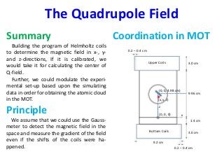
1. The Quadrupole Field
Summary
Building the program of Helmholtz coils
to determine the magnetic field in x-, y-
and z-directions, If it is calibrated, we
would take it for calculating the center of
Q-field.
Further, we could modulate the experi-
mental set-up based upon the simulating
data in order for obtaining the atomic cloud
in the MOT.
Principle
We assume that we could use the Gauss-
meter to detect the magnetic field in the
space and measure the gradient of the field
even if the shifts of the coils were ha-
ppened.
Coordination in MOT
1.4 cm
(0, 0, 0) x
z
9.96 cm
3.0 cm
3.0 cm
9.2 cm
0.2 – 0.4 cm
0.2 – 0.4 cm
(0, 0, 4.98 cm)
(x, y. z)
Upper Coils
Bottom Coils

2. Analyses
The magnetic fields for x-, y- and z- com-
ponents (Bx, By, Bz) would be compared
with them at the same position or near, as
the coils are shifted and not. These data
would present the gradient of the field and
lead us to know the direction where the
center of field moves towards, and the
procedures are as followed:
Firstly, we find the center of field
according to Bz when the coils do be fixed,
and z-position is 4.3 cm in the space leads
Bz is zero. [fig.1] and [fig.2].
Secondly, we make sure the z-position of
the field center in this case and do further
for Bx and By near the center in order for
understanding its gradient of the field.
[fig.3] and [fig.4].
fig.1: The Bz in the space
when z-shift is only.
fig.2: The Bz is measured
along the central z-axis wh-
en z-shift is only.
fig.3: The Bx
is measured
near the
central z-axis
when z-shift
is only.
fig.4: The By
is measured
near the
central z-axis
when z-shift
is only.

3. Thirdly, compared to the data that the
coils do be fixed w/o x-shift, we are able
to observe the variation of field at the
same positions when there are x-shift and
z-shift. In addition, we could predict
where the center of the field goes to.
[fig.5], [fig.6] and [fig.7].
Name Linearly Fitting
d(Bz)/dz
(G/cm)
Center (Original, x = 0 & y =0) Bz = -22.56z + 96.45 22.56
Center (Later, x = 0 & y = 0) Bz = -22.61z + 96.67 22.61
Negative (Later, x=-2.4 cm & y = 0) Bz = -24.06z + 101.8 24.06
Positive (Later, x = 2.4 cm & y = 0) Bz = -23.4z + 100.9 23.40
Obviously, there would be variation of
field less than 6.64 % when x-shifts are
0.4 cm to the upper and bottom coils
and MAYBE, the center would move to
the certain direction???? (I roughly de-
termined that the center of field might
move ±0.04 cm.)
Again, by the same way, we would
analyze the data to identify which
direction the center moves to and
determine the shift of the center as the
reference that we modulate the position
of insection of the MOT beam with the
center of the field.
fig.5: The Bz is
measured at
original and near
the central z-axis
when z-shift amd
x-shift were
happened..
fig.6: The Bx is measured fig.7: The By is measured

4. However, there is one problem
I am confused about how to define the
center of the field when the shifts were
happened. Specifically, if meeting the situ-
ation, atoms in the MOT would decide
which direction they move to by the gra-
dient of the field or the lest magnetic field
in the space?
Conclusions
We would scan where is near the original
center of the field in order for converging
the optical set-up of the MOT beam if the
program is close to the experimental para-
meters and the principle is clear as well.
In addition, if we really enhace the qua-
drupole field to move the center of the
field by Helmholtz coils, we could go ahead.