Mj3621112123

Rasul M. Khalaf et al Int. Journal of Engineering Research and Applications
ISSN : 2248-9622, Vol. 3, Issue 6, Nov-Dec 2013, pp.2111-2123

RESEARCH ARTICLE

www.ijera.com

OPEN ACCESS

Experimental and Artificial Neural Networks Modeling for Rivers
Bed Morphology Changes near Direct Water Supply Intakes
Rasul M. Khalaf 1 Rafa H. Al-Suhaili 2 Sanaa A. T. Al-Osmy3
1 Department of Civil Engineering, University of Al-Mustansiriyah, Baghdad, Iraq.
2 Department of Civil Engineering, University of Baghdad, Baghdad, Iraq.
Visiting Prof. , City College of New York. New York, USA.
3 Department of Civil Engineering, University of Al-Mustansiriyah, Baghdad, Iraq.

ABSTRACT
In this research, the problem of sediment movements near direct intakes was investigated from the river bed
morphology point of view rather than that concerning the effect of sediment withdrawal by the intake to the water
treatment plant. As expected the river bed morphology will be affected by the intake operation, and when the
pumping stops, the river will tend to recover this effect by its natural flow, hence a model is required to relate the
rate of river bed morphology recovery to the variables that are expected to be relevant, such as the pumping rate, the
geometrical variables and time of operation to time of non-operation ratio. A physical model was built. Experiments
were conducted to create a data base for these input-output variables, which were used to find an (ANN) model, for
the representation of this relationship. Image processing technique is used in this study to analyze the scour and
deposition photos from which the volumes of the scour holes after intake operation time and that after intake nonoperation time were found, which allows the estimation of the rate of recovery. The results obtained from the image
processing of these photos had prevailed that these volumes can be approximated as a half ellipsoid. An ANN.factorized back propagation model was fitted to the data base with a correlation coefficient of (0.843), which was
considered acceptable according to Smith (1986) criteria. Comparison between the output values(rate of recovery)
obtained using this (ANN) model and those obtained experimentally for cases that are not included in the data base,
indicates high compatibility with a maximum percentage difference of (7.15% and 5.07%) for overestimating and
underestimating respectively.
Keywords: River morphology, Souring, Sedimentation, Rate of recovery, Artificial Neural Networks, Water
intakes.

I.

INTRODUCTION

Sediment movement near the river intake
structures is a complex problem that reduces the system
efficiency and increases the cost of dredging and system
maintenance.
In case of power-plants using rivercooling water, sediment reduces the withdrawn capacity
of the plant, causes damage to the pumping system and
partial or full blockage at the entrance of intake.
Sediment blockage may result in the stopping of the
plant, Abd Al-Haleem, (2008).
As water is abstracted through the intake,
sediment is typically drawn towards the intake structure
or point of diversion. Sediment may either be drawn into
the intake structure or may be trapped behind it. This
reduces the amount of sediment that is supplied to
downstream reaches. If sediment is drawn into the
intake, there is the risk of damage to the intake facility
and end operation machinery (e.g. turbines, gates and
valves), Ali et al.(2012).
www.ijera.com

Many researches had been conducted
concerning the problem that occurs in the water supply
projects due to sediment withdrawal, Amin
(2005),Zheng and Alsaffar(2000). However, very little
work had been done on the effect of direct water intakes
operation on the river bed morphology, Formann et al.
(2012), Zaitsev et al.(2004). These intakes operation
can affect the river bed morphology by creating
considerable changes in the bed formation near the
intake, and disturb the river as a system. This operation
causes movement of sediments near the intake creating
some sort of a hole in the vicinity of the intake. Part of
the sediments moved due to pumping will be withdrawn
with the pumped water, while the other part will move
just downstream the intake where it deposited creating
local sediment accumulation. The reduction in sediment
downstream and increased erosion can damage
important habitats (e.g. bank-side habitat) and habitats

2111 | P a g e

that depend on a supply of sediment from upstream
reaches,SEPA (2008).
For a scientific and rational approach to
different river problems and proper planning and design
of water resources projects, an understanding of the
morphology and behavior of the river is a pre-requisite.
River morphology is a field of science which deals with
the change of river plan and cross sections due to
sedimentation and erosion. In this field, dynamics of
flow and sediment transport are the principal elements.
The morphological studies, therefore, play an important
role in planning, designing and maintaining river
engineering structures, Agrawl(2005).
These changes in the river morphology near the
intake may disturb the natural river system. It may have
effects on the natural flow and the ecosystem. However,
the river system will try to retain its natural properties
when the disturbance created by the water intake
operation stop. This is the recovery property of any
natural system such as rivers.
Artificial neural networks modeling had been
used for the modeling of scour phenomena at outlet
structures, Emamgholizadeh (2012). These models had
proved their capability of estimating the depth of scour
holes created by the flow around bridge piers, Jeng et al.
(2005).
In this research it is intended to look at the
problem of sediment movements near direct intakes
from the river bed morphology point of view rather than
those problems concerning the water treatment. The
reasons for this attention are due to the facts that little
researches had been conducted on this issue compared
to the concern of the water treatment problems, and that
so many direct intakes were already exist in Iraq and
still working. Exchanging these direct intakes into side
intakes is an expensive and impractical action, hence it
is believed that proper operation of these direct intakes
can minimize the effect on the river morphology.
The following main steps were conducted to
achieve the aim of the research.
1- Building a physical model, that simulates a direct
intake operation on a river.
2- Conduct experiments to establish a data base for the
set of data relating the rate of recovery of the river
bed material to the pumping rate and time schedule.

www.ijera.com

www.ijera.com

3- 3- Develop an artificial neural networks model for
relating the variables using the data base developed
in step2.

II.

THE EXPERMENTAL SETUP

A movable bed flume, re-circulating type was
built. Its parts are collected from different public
markets in Baghdad, Iraq, such as electrical pumps and
flow meters. The system is a closed operating system.
Figure (1) shows the general layout of the flume. The
flume is consisted of the following main parts:
Flume Body
The main flume is of 3m long and has a
rectangular cross-section (1.2 m x 1 m). The flume
structure is built up from iron and its sides and bed are
manufactured from 8 mm thickness acrylic material,
The entrance of the flume is provided with a stilling
basin with a fine mesh screen to ensure an even flow
distribution across the flume. At the downstream end of
the flume, there exists a rectangular Sharp crested weir
which has been manufactured to calculate the flume
(river) flow. The working section of the flume is 2.5m
length, 1.2m width and 1m in depth. This working
section is filled with 15cm thickness layer of natural
river soil taken from Tigris River.
Ground Tank with Re-circulating Pump
The ground tank was built using aluminum
material, has dimensions of (3 m x 1.20 m x 2 m). Water
is pumped from this tank to the flume, by means of two
centrifugal pumps each with a capacity of (280) lit/s.
The suction pipe of the centrifugal pump is (3) m long
and (0.33) m in diameter. It is submerged in the ground
tank to deliver water for the flume. Figure (2) shows the
ground tank and the re-circulating pump.
Intake Structure
The intake structure is made up of a suction
pump with a capacity of (500) lit/sec which was used to
withdraw water from the flume through the intake pipe
to the storage or ground tank. This pump is connected
with a UPVC pipe (1.25)" ,in diameter and (40)" ,in
length which works as an intake vertical pipe. This pipe
was submerged into the river (flume) and convey the
water to the flume (river) then finally to the ground tank
as shown in figure (3).

2112 | P a g e


www.ijera.com

Fig. (1) General layout of the flume

Fig.(2) Ground water storage tank and re-circulating pumps.

www.ijera.com

2113 | P a g e


www.ijera.com

Flow meter

Intake Pump

Intake Pipe

Fig. (3) Intake pump and flowmeter.
Flow meters
The inlet flow to the flume and outlet flow
from the intake pump were measured by using two
flow meters. One of them is connected to the flume

inlet pipe which was coming from the ground pumps
to measure the flume flow (QR) and the other is
connected to the intake pump to measure the intake
flow as shown in figure (4) .

Fig. (4) Ground flow meter and intake flow meter for measuring the intake discharge.
Point gauge
A Point gauge was installed within the flume
as shown in figure (5). A Carriage was constructed on
the two rails on the two sides of the main and intake
flumes. The carriage could be moved along the whole
length of the flume. The point gauge was fitted on the
www.ijera.com

carriage and used to measure both water and bed levels.
An industrial scraper was manufactured from an iron
material in order to be used for making a level bed
before each run. The point gauge was also used to
measure the bed topography on the working section of
the flume before each run.
2114 | P a g e


www.ijera.com

Fig. (5) The movable point gauge.
Digital Camera
A digital camera of (16Mega Pixel) was used
to monitor the bed topography on the whole working
section (2.5)m with a grid of (60 cm x 60 cm) around
the intake suction pipe. The photos were then analyzed
by using the image processing technique.

III.

EXPERIMENTAL PROGRAM

Experiments were carried out considering the
main parameters that affect the movement of the noncohesive sediments near the water intakes. The studied
effective parameters are as follows:-intake pumping flow, (Qp)
-River flow,(QR)
-horizontal position of the intake pipe, (d)
-width of the river(flume),(w)
-horizontal coordinate of any point along the river
flow direction,(x)
-length of river reach,(Lr)
-Transverse coordinate of any point along the direction
perpendicular to river flow direction (along the tank
widthdirection),(y)
- depth of sediments at any point (x,y),(z)
- Vertical position of the intake point,(dsn)
- Normal depth of river,(Yn)
- time of operation condition of the intake, top
- time of non-operation condition of the intake, tnop
The experimental tests are divided into many
different sets. For each set of experiments, different
ratios of ( Qr) i.e., (Qp/Qr) were used. For each value
of discharge ratio, different values of time ratios(tr)
i.e., (top/tnop) were used.

www.ijera.com

IV.

EXPERIMENTAL RESULTS
ANALYSIS

The analysis of the experimental results is
presented here for some of the experiments only for
the purpose of illustration. The given sample will
show the obtained scour hole after direct pumping and
the analysis of its photo using the image processing
technique. The recovery of scour hole after nonoperating stage is also shown here using the image
processing technique. Figure (6) shows a typical scour
hole photo and its image processing analysis. Figures
(7) and (8) show the scour hole and its image
processing before and after operation of the intake for
Qr=0.37,tr=0.33 , the estimated percentage recovery is
Pr=82.69%. All the photos of the other experimental
work runs were analyzed in a similar manner to that
shown in figures (7) and (8), using the image
processing technique. This technique can give the
dimensions of the scour hole after operation and nonoperation periods. The image processing technique can
also give the z- coordinate for the (x-y) coordinates of
any point on the scour hole. It also can draw a section
of the z- coordinates along any longitudinal line (x),
and/or transverse line (y), selected through the scour
hole section. For each photo of scour hole , relation
between x-y coordinates and depth z can be obtained
through the scour section . Table (1) represents the
depths (z) at different locations in a rectangular section
(60*60)cm, i.e., the z- coordinates for each 6 cm along
x and y directions of the section, for one of the images
analyzed.
Investigating all of the experimental results
had revealed that the shape of scour hole is similar to
a half of an ellipsoid, hence the volume of scour hole
can be approximated by the following formula:
2115 | P a g e

𝑉=
∗

1

2
4

π. Ls1. Ls2
. ds
Where:
Ls1=Horizontal axis of the ellipsoid.
Ls2=Vertical axis of the ellipsoid.
ds= central depth of scour hole.
3

(1)

Table (2) represents the obtained experimental results
for some experiments conducted. These data can be
classified into two parts:

www.ijera.com

1- The data which were measured during the
experiments such as (Yn, dsn,Qp, Qr, top and tnop).
2- The data obtained from the image processing
analysis of the scour holes volumes after pumping
operating and non-operating periods, (Vop, Vnop and
Pr%) ,which are the volume of hole after the operation
of intake, volume of hole after the period of nonoperation of the intake, and the percent recovery of the
hole, respectively. The percentage recovery is
estimated using the following equation:
𝑉𝑜𝑝 − 𝑉𝑛𝑜𝑝
𝑃𝑟 =
∗ 100
(2)
𝑉𝑜𝑝

Half of semiellipsoid
2
0
-2
-4
12
10
8

12
10

6

8

4

6
4

2
0

2
0

Fig. (6) A sample of a scour hole photo and its image processing after pumping operation time.

A)
B)
Fig. (7) A scour hole photos for (Qr=0.37,tr=0.33 , PR=82.69%), A) after pumping operation time period, B)
after non operation time period.

www.ijera.com

2116 | P a g e


www.ijera.com

2
0
-2
10
8
6
10
4

8
6
2

4
2
0

0

A)
B)
Fig. (8) Imag Processing for the Scour holes for (Qr=0.37,tr=0.33 , PR=82.69%), A) after pumping operation
time period, B) after non operation time period.
Table(1 ) Sample of the Image Processing Data results for a sample run.
X
1
2
3
4
5
6
Y
0.921
0.033
0.303
0.265
0.419
0.496
-0.352
0.651
0.033
-0.468

1
2
3
4
5
6
7
8
9
10

-0.275
-0.043
0.342
-0.120
0.265
0.728
0.651
0.728
0.574
-1.047

-0.082
-0.159
0.998
1.114
0.805
0.265
0.805
0.458
0.921
-0.54

0.303
-0.082
0.342
-0.082
0.535
-0.429
-0.236
0.342
0.033
-0.429

-0.506
-0.005
-0.043
0.767
-1.664
-1.626
-0.468
0.149
0.188
-0.198

-0.159
-0.236
0.110
-1.085
-0.854
-0.159
0.072
-0.622
-0.005
0.265

7

8

9

10

-0.005
0.535
-0.468
0.381
-0.120
0.033
0.496
0.767
0.612
-0.159

-0.622
-0.506
-0.120
-0.275
0.303
0.072
0.689
0.072
-0.545
-1.008

0.072
-0.699
0.188
0.574
0.612
0.458
0.419
-1.047
0.188
-0.506

-0.198
0.226
0.265
-0.005
0.381
0.188
-0.082
0.728
0.149
-0.506

Table (2) Sample of the measured experimental results.
Run No.

Qp
(m3/sec)

Qr
(m3/sec)

d
(cm)

W
(cm.)

dsn
(cm.)

Yn
(cm.)

top
(min.)

tnop
(min.)

1

4.1

5.83

32

120

18

22

9

25

2

3.35

5.8

32

120

21

22.5

9

20

3

3.53

6.33

29

120

16

19

13.5

40

4

3.19

7.614

27.5

120

14.5

17.5

27

50

5

3.19

4.68

27.5

120

10.5

14.5

15

30

6

2.91

3.86

34

120

13.5

17.2

33

60

7

3.05

4.76

34

120

14.2

18.2

25

90

8

2.23

2.84

34

120

13.3

18.3

21

35

www.ijera.com

2117 | P a g e


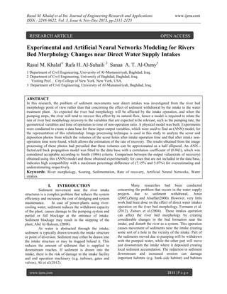
www.ijera.com

9

2.18

4.33

34

120

15.8

19.8

18

60

10

2.79

4.53

34

120

16.2

18.2

9

31

11

3.19

5.61

34

120

18.5

20

13

40

12

3.48

4.53

34

120

17

19

10

60

13

2.31

3.19

34

120

19

22

10.5

41

The Developed ANN Model
Using the data base developed in the
experimental work and ANN modeling technique,
different trials were made and finally an ANN.factorized back propagation model was obtained with
a correlation coefficient of (0.843), which was
considered acceptable according to smith(1986)
criteria. The input variables were changed to a
dimensionless terms to provide generality of the
model. These dimensionless variables are as follows:
dow=(d/w), the ratio of the horizontal position of the
intake pipe to the river width.
Qr=(Qp/QR), the ratio of the pumped discharges to
the river discharge.
tr=(top/tnop), the ratio of the time of operation of the
intake to time of non-operation.

dr=(dsn/yn), the ratio of the depth of the
submergence of the intake strainer to the normal
depth of the river.
These variables were used as input
variables, while the rate of recovery Pr is used as the
output variable. The SPSS (Statistical Procedures of
Social Sciences), version 19 was used for obtaining
the required ANN model.
Table (3) shows the data division, where the
application of (SPSS) software allows the selection of
this data division into training set, testing set, and
validation (holdout) set. The best data division that
was obtained is 79.2% (38Runs) for training, 8.3% (4
Runs) for testing, and 12.5% (6 Runs) for the
validation.

Table(3) Case Processing Summary.
Sample

Training
Testing
Holdout

Valid
Excluded
Total

N
38
4
6
48
0
48

Percent %
79.2
8.3
12.5
100

Table (4) shows the model network information, which indicates a number of hidden nodes in the hidden layer of
(7). The obtained required activation functions for the hidden and output layers were hyperbolic tangent and identity
functions respectively. Figure (9) shows the architecture of the network.
Table (4) Artificial neural network information.
Input Layer

www.ijera.com

1

dow

Covariates

Hidden Layer(s)

Factors

1
2
3

Qr
tr
dsn/yn
9
Standardized
1

Number of Units*
Rescaling Method for Covariates
Number of Hidden Layers

2118 | P a g e

Number of Units in Hidden Layer 1*
Activation Function
Dependent Variables
1

7
Hyperbolic tangent
Pr

Number of Units
Rescaling Method for Scale Dependents
Activation Function
Error Function

Output Layer

www.ijera.com

1
Standardized
Identity
Sum of Squares

*. Excluding the bias unit

Figure (9) The architecture of the artificial neural network (ANN) model required for the modeling of the
phenomena.
Table(5) shows the error analysis of the obtained ANN model. This table indicates low sum of square errors and
relative errors for each of the training, testing and verification subsets.
Table (5) Error analysis of the developed ANN model.
Training

Testing
Holdout

Sum of Squares Error
Relative Error
Stopping Rule Used
Training Time
Sum of Squares Error
Relative Error
Relative Error

3.654
0.197
1 consecutive step(s) with no decrease in error *
0:00:00.03
1.620
1.079
2.462

Dependent Variable: Pr
*. Error computations are based on the testing sample.
Table (6) shows the model parameters vectors and matrices obtained for the model. The correlation coefficient
between the predicted and measured percentage recovery is (0.843).
www.ijera.com

2119 | P a g e


www.ijera.com

Table (6) The ANN model Parameters.

Where: 𝑉𝑜𝑏𝑖𝑎𝑠 𝑝,1 , and 𝑉𝑛 ,𝑝 are the bias vector and
weight matrix between the input and hidden layers, p is
the number of hidden nodes in the hidden layer. For the
developed model, p=7 and the vector and matrix are as
given below:
−0.93
−0.548
−1.398
……(5)
𝑉𝑜𝑏𝑖𝑎𝑠 𝑝,1 = 𝑉𝑜𝑏𝑖𝑎𝑠7,1 = −0.766
−0.220
0.656
−0.023
𝑉𝑛,𝑝 =𝑉4,7 =
0.969 0.644 −0.1970.033−0.229 0.023 −0.551
1.498 1.159 0.693 0.031 0.042 −0.375 0.532
𝑎(1) 𝑎(2) 𝑎(3) 𝑎(4) 𝑎(5) 𝑎(6) 𝑎(7)
0.677−0.658 1.105 0.053−0.743 0.469 0.095
(6)
Where the vector a(i) , i=1 to 7 is given by table(7).

In order to use the developed ANN model for
estimating the rate of recovery for a given input data set
the model can be represented by the following steps:
1- Put the input variables (dow,Qr,tr and dsn/yn)
in a the input vector 𝑋 𝑖 and obtain a
standardized form column vector 𝑋 ∗ using
𝑛,1
the following equation:
𝑋 𝑖 − 𝑚𝑒𝑎𝑛𝑥 𝑖
𝑋∗ =
(3)
𝑖
𝑆𝑑𝑥 𝑖
Where: 𝑋 ∗ , and 𝑋 𝑖 are the standardized and
𝑖
normal input variables respectively,
i=1,2,….N, where N is the number of input variables
(N=4 for the developed model), and
𝑚𝑒𝑎𝑛 𝑥𝑖 , , 𝑆𝑑𝑥 𝑖 are the observed means and standard
deviations of the input variables.
2- Obtain the weighted input vector to the nodes
of the hidden layer 𝑍𝑖𝑛 𝑝,1 ,using the following
matrix equation:
𝑇
𝑍𝑖𝑛 𝑝,1 = 𝑉𝑜𝑏𝑖𝑎𝑠 𝑝,1 + 𝑉𝑛 ,𝑝 ∗ 𝑋 ∗
4
𝑛,1
Table(7) Values of (ai) vector related to (d/w) values.
d/w

a1

0.2292
0.2417
0.2583
0.2625
0.2667
0.2833

-0.096
-0.045
0.182
0.501
0.252
-1.287

www.ijera.com

a2

a3
0.956
-0.337
0.310
-0.527
0.041
0.886

a4

a5

a6

a7

0.487
-0.339
0.021
0.120
-0.874
-0.766

-0.456
-0.615
0.108
0.455
0.770
-0.036

-0.517
0.063
-0.174
0.244
0.195
0.146

0.862
-0.266
-0.101
0.574
0.318
0.073

-0.098
0.078
-0.397
0.199
0.347
0.385

2120 | P a g e


www.ijera.com

3- Obtain the output vector from the nodes of the hidden layer as follows:
𝑍𝑜𝑢𝑡 𝑝,1 = 𝐹ℎ 𝑍𝑖𝑛 𝑝,1 (7)
Where: Fh is the activation function of the hidden layer. This function for the developed model is a
hyperbolic tangent.
4- Obtain the input weighted vector to the nodes of the output layer, 𝑌𝑖𝑛 𝑚 ,1 using:
𝑇
𝑌𝑖𝑛 𝑚 ,1 = 𝑊𝑜𝑏𝑖𝑎𝑠 𝑚 ,1 + 𝑊𝑝,𝑚 ∗ 𝑍𝑜𝑢𝑡 𝑝,1
(8)
Where: 𝑊𝑜𝑏𝑖𝑎𝑠 𝑚 ,1 ,and 𝑊𝑝,𝑚 are the bias vector and weight matrix between the hidden and output
layers, m is the number of nodes in the output layer. For the developed model, m=1 and the vector and
matrix are as given below:
𝑊𝑜𝑏𝑖𝑎𝑠 𝑚 ,1 =𝑊𝑜𝑏𝑖𝑎𝑠1,1 = (-0.117)

(9)

−1.389
1.037
1.591
𝑊𝑝,𝑚 = 𝑊7,1 = −1.026
0.067
0.849
−0.378
5- Find the standardized output vector𝑌𝑜𝑢𝑡 ∗𝑚 ,1

(10)

𝑌𝑜𝑢𝑡 ∗𝑚 ,1 = 𝐹𝑜(𝑌𝑖𝑛) 𝑚 ,1
and then obtain the output variables using:
𝑌𝑗 ,1 = 𝑌𝑗 ∗ ∗ 𝑆𝑑𝑦 𝑚𝑗 + 𝑚𝑒𝑎𝑛𝑦 𝑗
,1

(11)
(12)

Where j=1,2,…m,. For the developed the
output variable is only one, since m=1, and that is the
value of Pr.
The reason for using the standardized variables
in the ANN model as shown in equations (3) and (12) is
that the model vectors and matrices parameters are
estimated using the standardized input and output
variables. This is usually recommended for ANN
modeling to avoid the effect of order of magnitude of
each variable on these parameters. However the SPSS
software allows four method of modeling for the input
variables, non-scaling, standardized, normalized and
adjusted normalized. The standardized scaling method
was used for the input data since it was found to
produce the higher correlation coefficient between the

predicted and observed output variable. For the output
variables, the software uses a standardization method
by default, i.e. the output values (Pr%) is not the real
values but the standardized values, hence using this
model, the output values should be returned to the real
values by multiplying by the standard deviation and
adding the mean of each output variables. This will
require also the calculation of a mean value and the
standard deviation (sd) for output variable (Pr%) which
will be used later for returning the real output values of
(Pr%).
The mean and standard deviation values are
needed for the model use as mentioned above, hence,
considered as a model parameters. Table (8) shows
these means an standard deviations.

Table (8) The means and standard deviations of the input-output variables.
Variable
Mean
Standard deviation

Qr

tr

d/w

dsn/Yn

Pr

0.617143
0.142285

0.319061
0.13545

0.26399
0.014037

0.892245
0.047778

62.6795
16.44976

Even though the ANN modeling process
involves the division of data into three sub-samples as
mentioned above, the training, testing and verification
sub samples, and obtaining the model parameters using
the first two sub-samples leaving the third sub-sample
for verification, further verification was made herein to
ensure the model performance. This further verification
was done using some additional experimental data that
www.ijera.com

are not used in the ANN modeling. Table (9) shows the
results of the observed and predicted rate of recovery of
these additional experiments. The maximum percentage
difference was found to be (7.15) overestimating and
(5.07) underestimating. This ensures the model good
performance. Hence this model can be used for design
and/or operation purposes for direct intakes on rivers.

2121 | P a g e

Designers and operators of such intake can use
this model to estimate the rate of recovery for proposed
or existing intake geometric and pumping capacity
variables. For example if the required daily pumping
volume is V and the proposed number of cycles per day
is nc, then:

𝑇𝑜𝑝 =

www.ijera.com

𝑉

(13)

𝑄𝑝

Top=nc (top+tnop)
𝑡𝑜𝑝
𝑡𝑟 =
𝑡𝑛𝑜𝑝

(14)
(15)

Table (9) Percentage difference between observed and estimated rate of recovery percent using the developed
ANN model.
Input Variables
Qr
0.703
0.5577
0.7539
0.7852
0.7741
0.7296
0.5114

tr
0.3600
0.3375
0.5500
0.6000
0.2561
0.5000
0.2500

d/w
0.2667
0.2417
0.2833
0.2833
0.2833
0.2583
0.2583

Output Variables
dsn/yn
0.8182
0.8421
0.8430
0.8361
0.8636
0.9444
0.9000

The designer and operators can use a trial and
error procedure by the following steps:
1- For the given V and 𝑄 𝑝 estimating Top from
equation(13)
2- Solving equations(14) and (15) to find tr for a
proposed values of nc and top.
3- Using the tr with the other proposed values as input
variables in the developed ANN model to obtain
the rate of recovery then repeating the process until
a satisfied rate of recovery is obtained.
Table(8) Independent Variable Importance analysis.
Variable number
Variable name

PR Observed
73.5331
67.0000
54.2210
40.1530
89.8600
77.2300
63.3000

PR Estimated
78.7900
70.1000
51.4700
39.6300
88.4140
73.7900
63.7900

% difference
-7.15
-4.69
5.07
1.30
1.62
4.46
-0.72

A relative normalized importance analysis was
performed in order to find which of the input variables
has the most effect on the output variable. Table (10)
shows the results which indicate the effect of input
variables in descending order as d/w, Qr, tr and ds/yn
respectively. The last three variables has almost the
same effect of approximately (60%) on the rate of
recovery.

Importance

Normalized importance

VAR00001

d/w

0.356

100%

VAR00002

Qr

0.216

60.7%

VAR00003

tr

0.219

61.6%

VAR00004

dsn/yn

0.209

58.71%

V.

CONCLUSIONS:

Form the experimental and analytical study
conducted above the following conclusions can be
deduced:
1- Photos should be taken by fixing the digital
camera at the same vertical location or level
during the experimental work. Different locations
of the camera will lead to different range of data
and will not help to make a precise comparison
between operation and non-operation behavior of
www.ijera.com

the river bed morphology. In addition to that
photos should be taken using the same digital
camera settings and the same section dimensions
for all of the experiments. Using different pixels
and section dimensions will lead to give different
range of data, which will not give a real
presentation of the phenomena under study.
2- The analysis of the results of the image processing
indicate the possibility of approximating the
volume of the created hole by measuring the
2122 | P a g e

principal axis of this hole and using the formula of
half ellipsoid volume.
3- Comparison between the rates of recovery values
obtained using the physical model with those
obtained using the developed (ANN) model
indicates high compatibility with a maximum
percentage difference of (7.15% and 5.07%) for
overestimating and underestimating respectively.
4- The normalized importance analysis indicates that
the ratio (d/w) has the highest effect on the rate of
recovery with normalized relative importance of
100%.The other three variables (Qr, tr, dsn/yn)
has almost the same normalized relative effect on
the rate of recovery, which is about 60%.
5- Using this modeling technique, different trials
were made and finally an (ANN.-factorized back
propagation model) was observed with a
correlation coefficient of (0.843), which was
considered acceptable according to smith criteria.
The reason for obtaining a factorized ANN model
rather than the traditional one is due to the fact
that (d/w) was found to have an effect on the
percent recovery as a factorized factor rather than
as a variable.

[7]

[8]

[9]

[10]

www.ijera.com

Scour Depth Around Bridge Piers", Research
Report No.R855, Department of Civil
Engineering, University of Sydney, Australia,
November
2005,
http://www.civil.usyd.edu.au/.
Scottish Environment Protection Agency
(SEPA), 2008 ,"Intakes And Outfalls" 1st
Edition, October 2008.
Smith, M. (1993), “Neural Networks for
Statistical Modeling”, Van NostrandReinhold, New York.
Zaitsev, A. A., Belikov, V.V. and Militeev,
A. N. ,2004" Sediment Transfer Through the
Fluvial System using Computer Modeling for
Regulation of Sediment Transport Under
Hydraulic Structures an A Large River ",
Proceedings of A Symposium Held In
Moscow, August 2004, IAHS Publ. 288,
pp.386-394.
Zheng, Y. and Alsaffar, A. M. ,2000,"
Water Intake Sediment Problems in Thermal
Power
Plants",
ASCE,
Doi:
10.1061/40517(2000)273 ,pp. 1-8.

REFERENCES
[1]

[2]

[3]

[4]

[5]

[6]

Abd Al-Haleem, F.S.F., 2008,"Sediment
Control At River Side Intakes", Ph.D Thesis,
Department of Civil Engineering, Faculty of
Engineering, Minufiya University ,Egypt.
Agrawal, A.K., 2005," Numerical Modeling
of Sediment Flow In Tala Desilting
Chamber" M. Sc. Thesis, Norwegian
University of Science and Technology,
Faculty of Engineering Science and
Technology, Department of Hydraulic and
Environmental Engineering, Norwig.
Ali, A. A., Al-Ansari N. A. and Knutsson, S. ,
2012 ," Morphology of Tigris River Within
Baghdad City", Journal of Hydrology and
Earth System Sciences., 16, pp.3783–3790.
Amin, A. M. A. , 2005,"Study Of
Sedimentation At River Side Intakes", Ph.D
Thesis, Minufiya University, Faculty Of
Engineering, Civil Engineering Department,
Shebin El-Kom, Egypt.
Emamgholizadeh, S., 2012," Neural Network
Modeling of Scour Cone Geometry Around
Outlet in The Pressure Flushing", Global
NEST Journal, Vol.14, No.4, pp. 540-549.
Jeng D-S, Bateni S. M., and Lockett
E.,(2005)," Neural Network Assessment For

www.ijera.com

2123 | P a g e

Mj3621112123

Recomendados

Recomendados

Mais conteúdo relacionado

Mais procurados

Mais procurados (18)

Destaque

Destaque (18)

Semelhante a Mj3621112123

Semelhante a Mj3621112123 (20)

Último

Último (20)

Mj3621112123