Modeling Job Shop Scheduling with Timed Petri Nets

Mullya Satish Anand, Santosh Krishnaji Sindhe / International Journal of Engineering
Research and Applications (IJERA) ISSN: 2248-9622 www.ijera.com
Vol. 3, Issue 2, March -April 2013, pp.492-496

Modeling and Simulation of Job Shop Scheduling Using Petri-
Nets
Mullya Satish Anand*, Santosh Krishnaji Sindhe**
*(Department of Mechanical Engg, IOK COE Pune)
** (Department of Mechanical Engg, IOK COE Pune)

ABSTRACT
In most of the manufacturing units to analyze the throughput of cyclic (production)
scheduling is a difficult task due to the complexity processes. Carlier, Chretienne & Girault (1984, 1988,
of the system. Hence powerful tools that can 1983), Gao, Wong & Ning (1991) and Watanabe &
handle both modeling and optimization are Ya-mauchi (1993) also focused on minimal cycle
required. Most of the research in this area focuses times for repetitive scheduling problems. In this
in either developing optimization algorithms, or in paper focus is on the traditional non-cyclic
modeling complex production systems. However, scheduling problems such as machine scheduling and
few tools are aimed to the integration of both of job shop scheduling (Pinedo, 1995). In this paper
them. In this paper, a Petri Net based integrated timed Petri net model is used and time is associated
approach, for simultaneously modeling and with transitions.
scheduling manufacturing systems, is proposed.
The procedure is illustrated with an example III. TIMED PETRI NETS
problem. Petri nets originate from the early work of
Keywords - Analysis of Petri Nets, INA, Petri Nets, Carl Adam Petri in 1962. Since then there has been
Scheduling. lot of research in study and application of Petri nets.
The classical Petri net is a bipartite directed graph
I. INTRODUCTION with two node types called places and transitions.
The prime subject of research on scheduling The nodes are connected via directed arcs. Two
problems consists of the optimal allocation of scarce nodes of the same type cannot be connected. Places
resources to tasks over time. Despite the complexity are represented by circles and transitions by
of many scheduling problems, effective algorithms rectangles. Places may contain zero or more tokens,
have been developed. However, most of research which are represented by black dots. The number of
focused on the effectiveness of the algorithms, tokens may change during the execution of the net.
neglecting the issue of flexibility. Research on Petri A place „p‟ is called an input place of a transition„t‟
nets addresses the issue of flexibility. To facilitate the if there exists a directed arc from p to t, p is called an
modeling of complex systems many extensions have output place of t if there exists a directed arc from t to
been proposed. Typical extensions are the addition of p. The net shown in Fig.I illustrate the classical Petri
„color‟, „time‟ and „hierarchy‟. These Petri nets have net model. These Petri net models a machine which
all the advantages of the classical Petri net, such as processes jobs and has two states free and busy.
the graphical nature, mathematical foundation and There are four places in, free, busy and out and two
the various analysis methods. Therefore, it is transitions start and finish. In the state shown in Fig.
interesting to investigate the application of Petri nets I there are five tokens; four in place in and one in
to scheduling. In this paper we concentrate on timed place free. The tokens in place in represent jobs to be
Petri nets, i.e. Petri nets extended with a timing processed by the machine. The token in place free
concept. indicates that the machine is free and ready to process
a job. If the machine is processing a job, then there
II. LITERATURE REVIEW are no tokens in free and there is one token in busy.
When Petri Nets were introduced, many The tokens in place out represent jobs which have
papers were published on topics such as resource been processed by the machine. Transition start has
utilization, bottlenecks, throughput, cycle times and two input places in and free and one output place
capacity estimations. Petri Nets were evaluated in busy. Transition finish has one input place busy and
manufacturing systems using different techniques two output places out and free. A transition is called
like simulation, queuing theory, probability and enabled if each of its input places contains at least
stochastic Petri nets. Most of the results in this area one token.
focused on cyclic scheduling problems.
Ramamoorthy & Ho (1980) and Hillion & Proth
(1989) have used a technique based on a „marked
graphs‟ (a subclass of Petri nets)

492 | P a g e


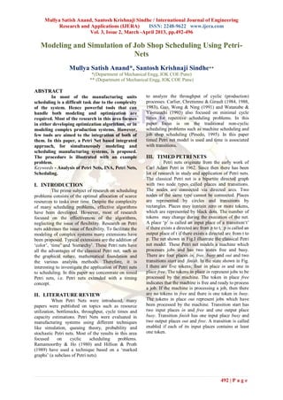
A timed Petri net is a six tuple TPN = (P, T, I, O, TS,
D) satisfying the following requirements:
(i) P is a finite set of places.
(ii) T is a finite set of transitions.
(iii) I ∈ T →P (P) is a function which defines the set
of input places of each transition.
(iv) O ∈ T →P (P) is a function which defines the set
of output places of each transition.
(v) TS is the time set.
(vi) D ∈ T → TS is a function which defines the
Figure I. A Petri net which represents a machine firing delay of each transition.
An enabled transition can fire. Firing a transition t The state of a timed Petri net is given by the
means consuming tokens from the input places and distribution of tokens over the places. Firing a
producing tokens for the output places, i.e. t „occurs‟. transition results in a new state. This way a sequence
Transition start is enabled in the state shown in of states M0, M1, .... Mn is generated such that M0 is
Fig. I, because each of the input places in and free the initial state and Mi+1 is the state reachable from
contains a token. Transition finish is not enabled Mi by firing a transition. Transitions are eager, i.e.
because there are no tokens in place busy . Therefore, they fire as soon as possible. If several transitions are
transition start is the only transition that can fire. enabled at the same time, then any of these transitions
Firing transition start means consuming two tokens, may be the next to fire. Therefore, in general, many
one from in and one from free, and producing one firing sequences are possible. Let M0 be the initial
token for busy. The resulting state is shown in Fig.II. state of a timed Petri net. A state is called a reachable
In this state only transition finish is enabled. Hence, state if and only if there exists a firing sequence M0,
transition finish fires and the token in place busy is M1, ...Mn which „visits‟ this state. A terminal state is
consumed and two tokens are produced, one for out a state where none of the transitions is enabled, i.e. a
and one for free. Now transition start is enabled, etc. state without successors.
As long as there are jobs waiting to be processed, the
two transitions fire alternately, i.e. the machine
IV. THE GENERAL SCHEDULING
modeled by this net can only process one job at a
time.
PROBLEM
Scheduling is concerned with the optimal
Timing Concept:
allocation of scarce resources to tasks over time.
To model the real systems it is often important to
Scheduling techniques are used in production
describe the behaviour of the system with the help of
planning, project planning, computer control,
durations and delays. Since the classical Petri net is
manpower planning etc.
not easily capable of handling quantitative time, we
Resources can be called as „machines‟ or
add a timing concept. In this paper a timing concept
„processors‟ and tasks as „operations‟ or „steps of a
is used where time is associated with transitions
job‟. Resources are used to process tasks. However, it
which determine delays. Firing is instantaneous, i.e.
is possible that the execution of a task requires more
the moment a transition consumes tokens from the
than one resource, i.e. a task is processed by a
input places the produced tokens appear in the output
resource set. There may be multiple resource sets that
places. However, because of the firing delay it takes
are capable of processing a specific task. The
some time before the produced tokens become
processing time of a task is the time required to
available for consumption. This results in the
execute the task given a specific resource set. By
following definition of a timed Petri net .
adding precedence constraints it is possible to
formulate requirements about the order in which the
tasks have to be processed. It is assumed that
resources are always available, but shall not
necessarily assume the same for tasks. Each task has
a release time, i.e. the time at which the task becomes
available for processing. This leads to the following
definition.
Definition 2
A scheduling problem is a six-tuple
SP = (T, R, PRE, TS, RT, PT) satisfying the
Figure II. Transition start has fired
following requirements.
(i) T is a finite set of tasks.
Definition 1
(ii) R is a finite set of resources.

493 | P a g e


(iii) PRE ⊆ T × T is a partial order, the precedence performed at the same time due to constraints on the
relation. usage of shared resources. Fig.III shows this
(iv) TS is the time set. structure. Here either transition t1 or t3 can be fired
(a) the resource sets capable of processing task t first. For example, a robot may be shared by two
and machines for loading and unloading.
(b) the processing time required to process t by a
specific resource set.

This definition specifies the data required to
formulate a scheduling problem. The tasks are
denoted by T and the resources are denoted by R. The
precedence relation PRE is used to specify
precedence constraints. If task t has to be processed
before task t‟, then (t, t‟) ∈ PRE, i.e. the execution of Figure III. Mutual Exclusive
task t has to be completed before the execution of In Fig. V places containing tokens indicate that jobs
task t‟ may start. TS is the time set. IN and IR+ ∪ {0} and machines are available initially. Processing times
are typical choices for TS. The release time RT (t) of are given to the transitions. TABLE III shows the
a task t specifies the time at which the task becomes transitions and its time. Other transitions given in the
available for processing, i.e. the execution of t may model apart from the transitions given in the table has
not start before time RT (t). 0 unit time. These transitions indicate start of the
process. T25 transition is a switch transition used to
Scheduling Problem: 3 jobs 4 machines problem complete the cycle; its time is 0 units. Initial state
Table I. Path of operations Table II. Time of consists of places P0, P1, P2 containing 1 token each
operations indicating start of job 1, 2 & 3. And final state
consists of places P38, P39, P40 containing 1 token
job 1 2 3 4 job 1 2 3 4 each indicating completion of job 1, 2, 3. To achieve
the final state transitions are fired according to
1 1 2 3 4 1 9 8 4 4 sequence of operations. The sequence of transitions
2 1 2 4 3 2 5 6 3 6 with minimum time is the optimum schedule.
Analysis of the Petri Net model is done with the help
3 3 1 2 4 3 10 4 9 2 of INA tool.

Table III. Transitions with time units
Above, TABLE I. shows path for operations which is
to be followed by 3 jobs and the TABLE II. shows T1 9 T6 4 T12 9 T18 2
the corresponding processing time of each job on a
particular machine.
T3 5 T8 8 T14 3 T20 4
Assumptions
1. No resource may process more than one task at a T4 10 T10 6 T16 4 T22 6
time.
2. Each resource is continuously available for
processing.
3. Each operation, once started, must be completed
V. INTEGRATED NET ANALYZER
With the help of INA, Petri nets of very
without interruptions.
4. The processing times are independent of the different kinds can be investigated under different
schedule. Moreover, the processing times are fixed firing rules (in particular timing) with regard to their
general properties. Properties which can be verified
and known in advance.
through the analysis are boundedness of places,
liveness of transitions, and reachability of markings
Fig. V shows Petri Net model of 3 job 4 machines.
or states.
The typical characteristics exhibited by the activities
INA combines the following: a textual editor for nets,
in a dynamic event-driven system, such as
a by-hand simulation part, a reduction part for
concurrency, decision making, conflict, sequentiality,
Place/Transition-
mutual exclusion, synchronization and priorities, can
be modeled effectively by Petri nets. Here mutual
exclusion is used to build the model. This is due to
the fact that 3 jobs may be ready to be processed with
a single machine, but as per our assumption machine
can process 1 job at a time. Mutually exclusive- Two
processes are mutually exclusive if they cannot be

494 | P a g e


Figure V. Petri Net model of 3 job 4 machines.

Figure VI. A Schedule for 3 jobs and 4 machines.

495 | P a g e


nets, an analysis part to compute: structural Computing Science, Eindhoven University of
information, place invariants, transition invariants, Technology.
reachability graphs. [3] Gonzalo Mejia, Nicholas G. Odrey “Job Shop
Scheduling in Manufacturing: An approach
using Petri Nets and Heuristic Search”.
[4] Tadao Murata “Petri Nets: Properties,
Analysis and Applications” Proceedings of
the IEEE, vol 77, no 4, 1989.
[5] Raida El Mansouri, Elhillali Kerkouche, and
Figure IV. Reachability Graph Allaoua Chaoui, “A Graphical Environment
Fig. IV shows Reachability Graph. The reachability for Petri Nets INA Tool Based on Meta-
graph of a timed Petri net is constructed as follows. Modelling and Graph Grammars”. World
We start with an initial state M. Then we calculate Academy of Science, Engineering and
all states reachable from M by firing a transition. Technology 44 2008.
Each node in the reachability graph corresponds to [6] Ramamoorthy, C.V. And G.S. H O (1980),
a reachable state and each arc corresponds to the Performance Evaluation of Asynchronous
firing of a transition. firing sequences. By Concurrent Systems Using Petri Nets, IEEE
computing the reachability graph, it is possible to Transactions on Software engineering 6,
analyze all possible For a net representing a 440–449.
scheduling problem, each of these firing sequences [7] Carlier , J., P. Chretienne , And C. Girault
corresponds to a feasible schedule. Therefore, (1984), Modelling scheduling problems with
reachability graph is used to generate many feasible Timed Petri Nets, in: G. Rozenberg (ed.),
schedules. Advances in Petri Nets 1984,Lecture Notes in
Computer Science 188, Springer-Verlag,
VI. RESULTS Berlin, 62–82.
INA is a textual tool whereas petri net is a [8] Hillion , H.P. And J.P Proth (1989),
graphical tool so the input to the INA tool is a Performance Evaluation of Job-Shop Systems
.PNT file which is in text form. INA gave all the Using Timed Event Graphs, IEEE
structural properties of the petri net model. INA Transactions on Automatic Control 34, 3–9.
computed reachability graph which consists of 34 [9] Pinedo,M. (1995), Scheduling: theory,
states and the optimum schedule was having a algorithms, and systems, Prentice-Hall,
make-span of 33 units. For this schedule the Engle-wood Cliffs.
sequence of firing of transitions is T4 T3 T1 T10
T16 T6 T8 T22 T12 T20 T14 T18. The Gantt chart
of the schedule is given in Fig. VI.

VII. CONCLUSION
The approach presented in this paper
shows that it is possible to model many scheduling
problems in terms of a timed Petri net. In fact, a
recipe has been formulated for mapping scheduling
problems onto timed Petri nets. This recipe shows
that the Petri net formalism can be used to model
tasks, resources and precedence constraints. By
mapping a scheduling problem onto a timed Petri
net, we are able to use Petri net theory to analyze
the scheduling problem. We can use Petri net based
analysis techniques to detect conflicting
precedence‟s, determine lower and upper bounds
for the minimal make-span, etc. By inspecting the
reachability graph, we can generate many feasible
schedules.

REFERENCES
[1] Jiacun Wang. “Petri Nets for Dynamic Event
– Driven System modeling.
[2] W.M.P van der Aalst. “Petri Net based
Scheduling” Department of Mathematics and

496 | P a g e

Modeling Job Shop Scheduling with Timed Petri Nets

Recomendados

Recomendados

Mais conteúdo relacionado

Mais procurados

Mais procurados (19)

Destaque

Destaque (20)

Semelhante a Modeling Job Shop Scheduling with Timed Petri Nets

Semelhante a Modeling Job Shop Scheduling with Timed Petri Nets (20)

Último

Último (20)

Modeling Job Shop Scheduling with Timed Petri Nets