IE-002 Control Chart For Variables

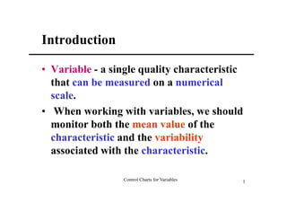
Introduction

• Variable - a single quality characteristic
that can be measured on a numerical
scale.
• When working with variables, we should
monitor both the mean value of the
characteristic and the variability
associated with the characteristic.

Control Charts for Variables 1

Control Charts for x and R (1)
Notation for variables control charts
• n - size of the sample (sometimes called a
subgroup) chosen at a point in time
• m - number of samples selected
• x i = average of the observations in the ith
sample (where i = 1, 2, ..., m)
• x = grand average or “average of the
averages (this value is used as the center
line of the control chart)

x and R(2)
Control Charts for
Notation and values
• Ri = range of the values in the ith sample
Ri = xmax - xmin
• R = average range for all m samples
•  is the true process mean
•  is the true process standard deviation


x and R(3)
Control Charts for
Statistical Basis of the Charts
• Assume the quality characteristic of interest is
normally distributed with mean , and standard
deviation, .
• If x1, x2, …, xn is a sample of size n, then he average of
x1  x 2    x n
this sample is
x
n
• x is normally distributed with mean, , and standard
deviation,
x   / n


Statistical Basis of the Charts
• The probability is 1 -  that any sample mean
will fall between

  Z  / 2 x    Z  / 2
n
and

  Z  / 2 x    Z  / 2
n
• The above can be used as upper and lower
control limits on a control chart for sample
means, if the process parameters are known.

x and R (5)
Control Charts for

x chart
Control Limits for the

UCL  x  A 2 R
Center Line  x
LCL  x  A 2 R
• A2 is found in Appendix VI for various values of
n.


Control Limits for the R chart

UCL  D4 R
Center Line  R
LCL  D3 R

• D3 and D4 are found in Appendix VI for various
values of n.

Estimating the Process Standard Deviation
• The process standard deviation can be
estimated using a function of the sample
average range.
Relative range： W=R/σ
R


E(W)=E(R/σ)=d2
d2
• This is an unbiased estimator of 


R=Wσ
Var(W)=d32

σR=d3σ
^
σR=d3(R/d2)


Trial Control Limits
• The control limits obtained from equations
should be treated as trial control limits.
• If this process is in control for the m samples
collected, then the system was in control in the
past.
• If all points plot inside the control limits and no
systematic behavior is identified, then the
process was in control in the past, and the trial
control limits are suitable for controlling
current or future production.

Control Charts for x and R(10)
Trial control limits and the out-of-control process
• If points plot out of control, then the control limits
must be revised.
• Before revising, identify out of control points and
look for assignable causes.
– If assignable causes can be found, then discard the point(s)
and recalculate the control limits.
– If no assignable causes can be found then 1) either discard
the point(s) as if an assignable cause had been found or 2)
retain the point(s) considering the trial control limits as
appropriate for current control. If future samples still
indicate control, then the unexplained points can probably
be safely dropped.

• Before revising, identify out of control points
and look for assignable causes.
– When many of the initial samples plot out of
control against the trial limits, (as few data will
remain which we can recompute reliable control
limits.) it is better to concentrate on the pattern
formed by these points.


• When setting up x and R control charts, it is
best to begin with the R chart. Because the
control limits on the x chart depend on the
process variability, unless process variability is
in control, these limits will not have much
meaning.


Example 5-1


Estimating Process Capability
• The x-bar and R charts give information
about the capability of the process
relative to its specification limits.


The fraction of nonconforming of
Example 5-1
• Assumes a stable process.
• Assume the process is normally
distributed, and x is normally distributed,
the fraction nonconforming can be found
by solving: P(x < LSL) + P(x > USL)


製程能力(process capability)
• 意義
– 對於穩定之製程所持有之特定成果，能夠合
理達成之能力界限。
• 製程能力的表示法
– 製程準確度(Ca值)
– 製程精密度(Cp值)製程能力比(process
capability ratio，PCR)
– 製程能力指數(Cpk值)


製程準確度Ca
(capability of accuracy)
製程平均值-規格中心值
Ca=
規格公差/2
=
X-μ
= T/2

T：規格公差=規格上限-規格下限


製程準確度之評價方法
• A級
– 小於等於12.5%理想的狀態，故維持現狀。
• B級
– 大於12.5%，小於等於25%儘可能調整改進至A級。
• C級
– 大於25%，小於等於50%應立即檢討並加以改善
• D級
– 大於50%，小於100%採取緊急措施，並全面檢討，
必要時應考停止生產。


製程精密度Cp
(process capability ratio，PCR)
雙邊規格：
規格公差 T
Cp= 6個估計標準差 = 6σ

單邊規格：
=
規格上限-製程平均值 SU-X
=
Cp= 3σ
3個估計標準差
或 =
製程平均值-規格下限 X-SL
=
Cp= 3σ
3個估計標準差

製程精密度評價方式
• A+級
– 大於等於1.67可考慮放寛產品變異，尋求管理的簡單化或成
本降低方法。
• A級
– 小於1.67，大於等於1.33理想的狀態，故維持現狀。
• B級
– 小於1.33，大於等於1.00確實進行製程管制，儘可能改善為
A級。
• C級
– 小於1.00，大於等0.67產生不良品，產品須全數選別，並管
理改善製程。
• D級
– 小於0.67採取緊急對策，進行品質改善，探求原因並重新檢
討規格。


製程能力指數Cpk

Cpk=(1-|Ca|)Cp
= =
X-SL
SU-X
Cpk=min{ }
3σ ， 3σ

當Ca=0時Cpk=Cp


製程能力指數評價方式
• A級
– 大於等於1.33製程能力足夠
• B級
– 小於1.33，大於等於1.00能力尚可應再努
力
• C級
– 小於1.00應加以改善


Process Capability Ratios (Cp)
(assume the process is centered at the
midpoint of the specification band)

If Cp > 1, then a low number of nonconforming
items will be produced.
• If Cp = 1, (assume norm. dist) then we are
producing about 0.27% nonconforming.
• If Cp < 1, then a large number of
nonconforming items are being produced.


The percentage of the specification band


ˆ   1 100%
P
C 
 p

**The Cp statistic assumes that the process mean
is centered at the midpoint of the specification
band – it measures potential capability.


Revision of Control Limits and Center Line
• The effective use of control chart will require
periodic revision of the control limits and
center lines.
– Every week, every month, or every 25, 50, or 100
samples.
– When revising control limits, it is highly desirable to
use at least 25 samples or subgroups in computing
control limits.
• If the R chart exhibits control, the center line of
the X Chart will be replaced with a target value.
This can be helpful in shifting the process
average to the desired value.

Phase II Operation of Charts
• Use of control chart for monitoring
future production, once a set of reliable
limits are established, is called phase II of
control chart usage
• A run chart showing individuals
observations in each sample, called a
tolerance chart or tier diagram, may
reveal patterns or unusual observations
in the data

Control Limits, Specification Limits,
and Natural Tolerance Limits(1)

• Control limits are functions of the
natural variability of the process
• Natural tolerance limits represent the
natural variability of the process (usually
set at 3-sigma from the mean)
• Specification limits are determined by
developers/designers.


• There is no mathematical relationship
between control limits and specification
limits.
• Do not plot specification limits on the
charts
– Causes confusion between control and
capability
– If individual observations are plotted, then
specification limits may be plotted on the
chart.

Rational Subgroups
• X bar chart monitors the between sample
variability (variability in the process over
time).
– Sample should be selected in such a way that
maximizes the chances for shifts in the process
average to occur between samples.
• R chart monitors the within sample variability
(the instantaneous process variability at a
given time).
– Samples should be selected so that variability within
samples measures only chance or random causes.

Guidelines for the Design of the
Control Chart(1)
• Specify sample size, control limit width, and
frequency of sampling
• if the main purpose of the x-bar chart is to
detect moderate to large process shifts, then
small sample sizes are sufficient (n = 4, 5, or 6)
• if the main purpose of the x-bar chart is to
detect small process shifts, larger sample sizes
are needed (as much as 15 to 25)…which is
often impractical…alternative types of control
charts are available for this situation…see
Chapter 8

Control Chart(2)
• If increasing the sample size is not an option, then
sensitizing procedures (such as warning limits) can
be used to detect small shifts…but this can result
in increased false alarms.
• R chart is insensitive to shifts in process standard
deviation for small samples. The range method
becomes less effective as the sample size increases,
for large n, may want to use S or S2 chart.
• The OC curve can be helpful in determining an
appropriate sample size.


Control Chart(3)
Allocating Sampling Effort
• Choose a larger sample size and sample less
frequently? or, Choose a smaller sample size and
sample more frequently?
• The method to use will depend on the situation. In
general, small frequent samples are more desirable.
• For economic considerations, if the cost associated
with producing defective items is high, smaller,
more frequent samples are better than larger, less
frequent ones.

Control Chart(4)
• If the rate of production is high, then more
frequent sampling is better.
• If false alarms or type I errors are very
expensive to investigate, then it may be best
to use wider control limits than three-sigma.
• If the process is such that out-of-control
signals are quickly and easily investigated
with a minimum of lost time and cost, then
narrower control limits are appropriate.

x
Changing Sample Size on the
and R Charts1
• In some situations, it may be of interest to
know the effect of changing the sample
size on the x-bar and R charts. Needed
information:
– Variable sample size.
– A permanent change in the sample size
because of cost or because the process has
exhibited good stability and fewer resources
are being allocated for process monitoring.


x
and R Charts2
• = average range for the old sample size
R old
• R new = average range for the new sample size
• nold = old sample size
• nnew = new sample size
• d2(old) = factor d2 for the old sample size
• d2(new) = factor d2 for the new sample size


x
and R Charts3
Control Limits
R  chart
x  chart
 d ( new ) 
UCL  D 4  2
 d 2 (new )   R old
UCL  x  A 2   d 2 ( old ) 
 R old
 d 2 (old)   d ( new ) 
CL  R new   2  R old
 d 2 (new )   d 2 ( old ) 
LCL  x  A 2   R old  
 d 2 ( new ) 
 d 2 (old)  UCL  max  0 , D 3   R old 
 d 2 ( old ) 
 

A2、D3、D4 are selected for the new sample size

Example 5-2


Charts Based on Standard Values
• If the process mean and variance are
known or can be specified, then control
limits can be developed using these values:
X  chart R  chart
UCL  D 2 
UCL    A 
CL  d 2 
CL  
LCL  D 1 
LCL    A 

• Constants are tabulated in Appendix VI


x and R Charts
Interpretation of
• In interpreting patterns on the X bar chart,
we must first determine whether or not the
R chart is in control.
• Patterns of the plotted points will provide
useful diagnostic information on the process,
and this information can be used to make
process modifications that reduce variability.
– Cyclic Patterns
– Mixture
– Shift in process level
– Trend
– Stratification Control Charts for Variables 44

x
The Effects of Nonnormality
• In general, the X bar chart is insensitive
(robust) to small departures from
normality.
• In most cases, samples of size four or five
are sufficient to ensure reasonable
robustness to the normality assumption.


The Effects of Nonnormality R1

• The R chart is more sensitive to
nonnormality than the x chart
• For 3-sigma limits, the probability of
committing a type I error is 0.00461on
the R-chart. (Recall that for x , the
probability is only 0.0027).


The Operating
Characteristic Function(1)
• How well the x and R charts can detect process
shifts is described by operating characteristic
(OC) curves.
• Consider a process whose mean has shifted
from an in-control value by k standard
deviations. If the next sample after the shift
plots in-control, then you will not detect the
shift in the mean. The probability of this
occurring is called the -risk.

The Operating
• The probability of not detecting a shift in the
process mean on the first sample is

   ( L  k n )   ( L  k n )
L= multiple of standard error in the control
limits
k = shift in process mean (#of standard
deviations).


The Operating
• The operating characteristic curves are plots of
the value  against k for various sample sizes.


The Operating
• If  is the probability of not detecting the
shift on the next sample, then 1 -  is the
probability of correctly detecting the shift
on the next sample.


Average run length，ARL
In-control
ARL0=1/α

Out-of-control
ARL1=1/(1-)


Average time to signal，ATS
and
Expected number of individual units
sampled，I

ATS=ARLh

I=nARL


Construction and Operation
of x and S Charts(1)

• First, S2 is an “unbiased” estimator of 2
• Second, S is NOT an unbiased estimator
of 
• S is an unbiased estimator of c4 
where c4 is a constant
• The standard deviation of S is  1  c 2
4


• If a standard  is given the control limits
for the S chart are:
UCL  B6
CL  c4
LCL  B5
• B5, B6, and c4 are found in the Appendix
for various values of n.

No Standard σGiven
• If  is unknown, we can use an average
1m
sample standard deviation, S   Si
m i1
UCL B4S
CL S
LCL B3S

x Chart when Using S
The upper and lower control limits for the x chart
are given as
UCL  x  A 3 S
CL  x
LCL  x  A 3 S

where A3 is found in the Appendix

Estimating Process Standard Deviation
• The process standard deviation,  can be
estimated by
S


c4


Example 5-3


The x and S Control Charts
with Variable Sample Size(1)
• The x and S charts can be adjusted to
account for samples of various sizes.
• A “weighted” average is used in the
calculations of the statistics.
m = the number of samples selected.
ni = size of the ith sample


with Variable Sample Size(2)
• The grand average can be estimated as:
m

n x i i
x i 1
m

n i
i 1
• The average sample standard deviation is:
1/ 2
 2
m

  ni  1Si 
S   i1m 
 ni  m 
 
 i1 

with Variable Sample Size
• Control Limits
UCL  x  A3S UCL  B 4 S
CL  x CL  S
LCL  x  A3S LCL  B 3 S

• If the sample sizes are not equivalent for each sample,
then
– there can be control limits for each point (control
limits may differ for each point plotted)

The S2 Control Chart

• There may be situations where the process
variance itself is monitored. An S2 chart is
S2 2
UCL    / 2,n 1
n 1
CL  S 2
S2 2
LCL  1(  / 2),n 1
n 1

  / 2 , n  1 and 1 (  / 2 ),n 1 are points found
2 2
where
from the chi-square distribution.

The Shewhart Control Chart
for Individual Measurements(1)
• What if you could not get a sample size greater than 1 (n
=1)? Examples include
– Automated inspection and measurement technology is
used, and every unit manufactured is analyzed. There is
no basis for rational subgrouping.
– The production rate is very slow, and it is inconvenient
to allow samples sizes of N > 1 to accumulate before
analysis
– Repeat measurements on the process differ only because
of laboratory or analysis error, as in many chemical
processes.
• The X and MR charts are useful for samples of sizes
n = 1.

個別值與移動全距管制圖(2)
• 使用理用
產品需經很久的時間才能製造完成
–
分析或測定一件產品的品質較為麻煩且費時
–
產品係非常貴重的物品
–
產品品質頗為均勻(自動化生產)
–
屬破壞性試驗
–
在於管制製造條件如溫度、壓力、濕度等
–


Moving Range Chart
• The moving range (MR) is defined as the
absolute difference between two
successive observations:
MRi = |xi - xi-1|
which will indicate possible shifts or
changes in the process from one
observation to the next.

X and Moving Range Charts
• The X chart is the plot of the individual
observations. The control limits are
MR
UCL  x  3
d2
CL  x
MR
LCL  x  3
d2
m
 MRi
where MR  i1
m



X and Moving Range Charts
• The control limits on the moving range
chart are:
UCL D4 MR
CL  MR
LCL 0


Example 5-5


Example
Ten successive heats of a steel alloy are tested
for hardness. The resulting data are
Heat Hardness Heat Hardness
1 52 6 52
2 51 7 50
3 54 8 51
4 55 9 58
5 50 10 51

Example
I and MR Chart for hardness

62 3.0SL=60.97
Individuals

X=52.40
52

-3.0SL=43.83
42
Observation 0 1 2 3 4 5 6 7 8 9 10

3.0SL=10.53
10
Moving Range

5
R=3.222

0 -3.0SL=0.000


Interpretation of the Charts
• X Charts can be interpreted similar to x charts. MR
charts cannot be interpreted the same as x or R charts.
• Since the MR chart plots data that are “correlated”
with one another, then looking for patterns on the
chart does not make sense.
• MR chart cannot really supply useful information
about process variability.
• More emphasis should be placed on interpretation of
the X chart.

Average Run Lengths
β
Size of Shift ARL1
1σ 0.9772 43.96
2σ 0.8413 6.03
3σ 0.5000 2.00
The ability of the individuals control
chart to detect small shifts is very poor.

Normal ProbabilityPlot
• The normality
assumption is often .999
.99

taken for granted. .95

lity
.80

Probabil
• When using the .50
.20

individuals chart, the .05
.01

normality .001

assumption is very 50 51 52 53 54 55 56 57 58
hardness
important to chart Average: 52.4 Anderson-Darling Normality Test
StDev: 2.54733 A-Squared: 0.648
N: 10 P-Value: 0.063

performance.

IE-002 Control Chart For Variables

Recomendados

Recomendados

Mais conteúdo relacionado

Mais procurados

Mais procurados (20)

Destaque

Destaque (20)

Semelhante a IE-002 Control Chart For Variables

Semelhante a IE-002 Control Chart For Variables (20)

Mais de handbook

Mais de handbook (20)

Último

Último (20)

IE-002 Control Chart For Variables