1. MATLAB 6.5 Image Processing Toolbox Tutorial
The purpose of this tutorial is to gain familiarity with MATLAB’s Image Processing
Toolbox. This tutorial does not contain all of the functions available in MATLAB. It is
very useful to go to HelpMATLAB Help in the MATLAB window if you have any
questions not answered by this tutorial. Many of the examples in this tutorial are
modified versions of MATLAB’s help examples. The help tool is especially useful in
image processing applications, since there are numerous filter examples.
1. Opening MATLAB in the microcomputer lab
1.1. Access the Start Menu, Proceed to Programs, Select MATLAB 6.5 from the
MATLAB 6.5 folder
--OR-1.2. Open through C:MATLAB6p5binwin32matlab.exe
2. MATLAB
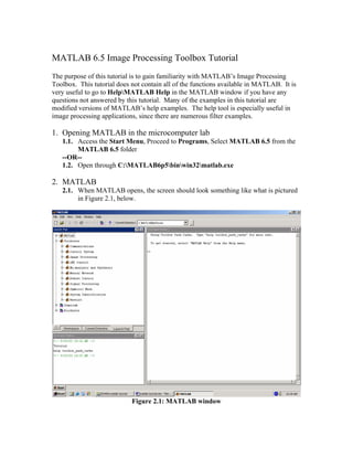
2.1. When MATLAB opens, the screen should look something like what is pictured
in Figure 2.1, below.
Figure 2.1: MATLAB window

2. 2.2. The Command Window is the window on the right hand side of the screen.
This window is used to both enter commands for MATLAB to execute, and to
view the results of these commands.
2.3. The Command History window, in the lower left side of the screen, displays
the commands that have been recently entered into the Command Window.
2.4. In the upper left hand side of the screen there is a window that can contain three
different windows with tabs to select between them. The first window is the
Current Directory, which tells the user which M-files are currently in use. The
second window is the Workspace window, which displays which variables are
currently being used and how big they are. The third window is the Launch
Pad window, which is especially important since it contains easy access to the
available toolboxes, of which, Image Processing is one. If these three windows
do not all appear as tabs below the window space, simply go to View and select
the ones you want to appear.
2.5. In order to gain some familiarity with the Command Window, try Example 2.1,
below. You must type code after the >> prompt and press return to receive a
new prompt. If you write code that you do not want to reappear in the
MATLAB Command Window, you must place a semi colon after the line of
code. If there is no semi colon, then the code will print in the command
window just under where you typed it.
Example 2.1
>> X = 1;
>> Y = 1;
>> Z = X + Y
%press enter to go to next line
%press enter to go to next line
%press enter to receive result
As you probably noticed, MATLAB gave an answer of Z = 2 under the last line
of typed code. If there had been a semi colon after the last statement, the
answer would not have been printed. Also, notice how the variables you used
are listed in the Workspace Window and the commands you entered are listed in
the Command History window. If you want to retype a command, an easy way
to do this is to press the ↑ or ↓ arrows until you reach the command you want to
reenter.
3. The M-file
3.1. M-file – An M-file is a MATLAB document the user creates to store the code
they write for their specific application. Creating an M-file is highly
recommended, although not entirely necessary. An M-file is useful because it
saves the code the user has written for their application. It can be manipulated
and tested until it meets the user’s specifications. The advantage of using an Mfile is that the user, after modifying their code, must only tell MATLAB to run
the M-file, rather than reenter each line of code individually.
3.2. Creating an M-file – To create an M-file, select FileNew ►M-file.
3.3. Saving – The next step is to save the newly created M-file. In the M-file
window, select FileSave As… Choose a location that suits your needs, such as
a disk, the hard drive or the U drive. It is not recommended that you work from

3. your disk or from the U drive, so before editing and testing your M-file you may
want to move your file to the hard drive.
3.4. Opening an M-file – To open up a previously designed M-file, simply open
MATLAB in the same manner as described before. Then, open the M-file by
going to FileOpen…, and selecting your file. Then, in order for MATLAB to
recognize where your M-file is stored, you must go to FileSet Path… This
will open up a window that will enable you to tell MATLAB where your M-file
is stored. Click the Add Folder… button, then browse to find the folder that
your M-file is located in, and press OK. Then in the Set Path window, select
Save, and then Close. If you do not set the path, MATLAB may open a
window saying your file is not in the current directory. In order to get by this,
select the “Add directory to the top of the MATLAB path” button, and hit
OK. This is essentially the same as setting the path, as described above.
3.5. Writing Code – After creating and saving your M-file, the next step is to begin
writing code. A suggested first move is to begin by writing comments at the top
of the M-file with a description of what the code is for, who designed it, when it
was created, and when it was last modified. Comments are declared by placing
a % symbol before them. Comments appear in green in the M-file window. See
Figure 3.1, below, for Example 3.1.
Example 3.1.
Run Button
Figure 3.1: Example of M-file
3.6. Resaving – After writing code, you must save your work before you can run it.
Save your code by going to FileSave.
3.7. Running Code – To run code, simply go to the main MATLAB window and
type the name of your M-file after the >> prompt. Other ways to run the M-file
are to press F5 while the M-file window is open, select DebugRun, or press
the Run button (see Figure 3.1) in the M-file window toolbar.

4. 4. Images
4.1. Images – The first step in MATLAB image processing is to understand that a
digital image is composed of a two or three dimensional matrix of pixels.
Individual pixels contain a number or numbers representing what grayscale or
color value is assigned to it. Color pictures generally contain three times as
much data as grayscale pictures, depending on what color representation scheme
is used. Therefore, color pictures take three times as much computational
power to process. In this tutorial the method for conversion from color to
grayscale will be demonstrated and all processing will be done on grayscale
images. However, in order to understand how image processing works, we will
begin by analyzing simple two dimensional 8-bit matrices.
4.2. Loading an Image – Many times you will want to process a specific image,
other times you may just want to test a filter on an arbitrary matrix. If you
choose to do this in MATLAB you will need to load the image so you can begin
processing. If the image that you have is in color, but color is not important for
the current application, then you can change the image to grayscale. This makes
processing much simpler since then there are only a third of the pixel values
present in the new image. Color may not be important in an image when you
are trying to locate a specific object that has good contrast with its surroundings.
Example 4.1, below, demonstrates how to load different images.
Example 4.1.
In some instances, the image in question is a matrix of pixel values. For
example, you may need something to test a filter on, but you do not yet need a
real image to test the filter. Therefore, you can simply create a matrix that has
the characteristics wanted, such as areas of high and low frequency. See
Example 6.1, for a demonstration of this. Other times a stored image must be
imported into MATLAB to be processed. If color is not an important aspect
then rgb2gray can be used to change a color image into a grayscale image. The
class of the new image is the same as that of the color image. As you can see
from the example M-file in Figure 4.1, MATLAB has the capability of loading
many different image formats, two of which are shown. The function imread is
used to read an image file with a specified format. Consult imread in
MATLAB’s help to find which formats are supported. The function imshow
displays an image, while figure tells MATLAB which figure window the image
should appear in. If figure does not have a number associated with it, then
figures will appear chronologically as they appear in the M-file. Figures 4.2,
4.3, 4.4 and 4.5, below, are a loaded bitmap file, the image in Figure 4.2
converted to a grayscale image, a loaded JPEG file, and the image in Figure 4.4
converted to a grayscale image, respectively. The images used in this example
are both MATLAB example images. In order to demonstrate how to load an
image file, these images were copied and pasted into the folder denoted in the
M-file in Figure 4.1. In Example 7.1, later in this tutorial, you will see that
MATLAB images can be loaded by simply using the imread function.
However, this function will only load an image stored in:

5. C:MATLAB6p5toolboximagesimdemos. Therefore, it is a good idea to
know how to load any image from any folder.
Figure 4.1: M-file for Loading Images
Figure 4.2: Bitmap Image
Figure 4.3: Grayscale Image

6. Figure 4.4: JPEG Image
4.3
Figure 4.5: Grayscale Image
Writing an Image – Sometimes an image must be saved so that it can be
transferred to a disk or opened with another program. In this case you will want
to do the opposite of loading an image, reading it, and instead write it to a file.
This can be accomplished in MATLAB using the imwrite function. This
function allows you to save an image as any type of file supported by
MATLAB, which are the same as supported by imread. Example 4.2, below,
contains code necessary for writing an image.
Example 4.2
In order to save an image you must use the imwrite function in MATLAB. The
M-file in Figure 4.6 contains code for saving an image. This M-file loads the
same bitmap file as described in the M-file pictured in Figure 4.1. However,
this new M-file saves the grayscale image created as a JPEG image. Just like in
Example 4.1, the “splash2” bitmap picture must be moved into MATLAB’s
work folder in order for the imread function to find it. When you run this Mfile notice how the JPEG image that was created is saved into the work folder.

7. Figure 4.6: M-file for Saving an Image
5. Image Properties
5.1. Histogram – A histogram is bar graph that shows a distribution of data. In
image processing histograms are used to show how many of each pixel value
are present in an image. Histograms can be very useful in determining which
pixel values are important in an image. From this data you can manipulate an
image to meet your specifications. Data from a histogram can aid you in
contrast enhancement and thresholding. In order to create a histogram from an
image, use the imhist function. Contrast enhancement can be performed by the
histeq function, while thresholding can be performed by using the graythresh
function and the im2bw function. See Example 5.1, for a demonstration of
imhist, imadjust, graythresh, and im2bw. If you want to see the resulting
histogram of a contrast enhanced image, simply perform the imhist operation
on the image created with histeq.
5.2. Negative – The negative of an image means the output image is the reversal of
the input image. In the case of an 8-bit image, the pixels with a value of 0 take
on a new value of 255, while the pixels with a value of 255 take on a new value
of 0. All the pixel values in between take on similarly reversed new values.
The new image appears as the opposite of the original. The imadjust function
performs this operation. See Example 5.1 for an example of how to use
imadjust to create the negative of the image. Another method for creating the
negative of an image is to use imcomplement, which is described in Example
7.5.
Example 5.1
In this example the JPEG image created in Example 4.2 was used to create a
histogram of the pixel value distribution and a negative of the original image.
The contrast was then enhanced and finally the image was transformed into a
binary image according to a certain threshold value. Figure 5.1, below, contains
the M-file used to perform these operation. Figure 5.2 contains the histogram of

8. the image pictured in Figure 4.3. As you can see the histogram gives a
distribution between 0 and 1. In order to find the exact pixel value, you must
scale the histogram by the number of bits representing each pixel value. In this
case, this is an 8-bit image, so scale by 255. As you can see from the histogram,
there is a lot of black and white in the image. Figure 5.3 contains the negative
of the image pictured in Figure 4.3. Pixel values have been rotated about the
midpoint in the histogram. Figure 5.4 contains a contrast enhanced version of
the image in Figure 4.3. As you can see, there is some blurring around the
edges of the object in the center of the image. However, it is slightly easier to
read the words in the image. This is an example of the trade-offs that are
common in image processing. In this case, sacrificing fine edges allowed us to
see the words better. Figure 5.5 contains a binary image of the image in Figure
4.3. This particular binary image was created according to the threshold level,
thresh. The value for thresh was displayed in the MATLAB Command Window
as:
>>
thresh =
0.5020
MATLAB chooses a value for thresh that minimizes the intraclass variance of
black and white pixels. If this value does not meet your expectations, use a
different value when using the im2bw function. Another function new to this
example was im2double. This function converts the image from its current
class to class double. Many MATLAB functions cannot perform operations on
class unit8 or unit16, so they must first be converted into class double. This is
due to the unsigned nature of class unit. Certain mathematical functions must
be able to output to a floating point array in order to operate. When writing an
image, MATLAB converts the data back to class unit.

9. Figure 5.1: M-file for Creating Histogram, Negative, Contrast Enhanced and
Binary Images from the Image Created in Example 4.2
Figure 5.2: Histogram
Figure 5.3: Negative
Figure 5.4: Contrast Enhanced
Figure 5.5: Binary
6. Frequency Domain
6.1. Fourier Transform – In order to understand how different image processing
filters work, it is a good idea to begin by understanding what frequency has to
do with images. An image is in essence a two dimensional collection of discrete
signals. Therefore, the signals have frequencies associated with them. For
instance, if there is relatively little change in grayscale values as you scan across
an image, then there is lower frequency content contained within the image. If
there is wide variation in grayscale values across an image then there will be
more frequency content associated with the image. This may seem somewhat
confusing, so let us think about this in terms that are more familiar to us. From

10. signal processing, we know that any signal can be represented by a collection of
sine waves of differing frequencies, magnitudes and phases. This
transformation of a signal into its constituent sinusoids is known as the Fourier
Transform. This collection of sine waves can potentially be infinite, if the
signal is difficult to represent, but is generally truncated at a point where adding
more signals does not significantly improve the resolution of the recreation of
the original signal. In digital systems, we use a Fourier Transform designed in
such a way that we can enter discrete input values, specify our sampling rate,
and have the computer generate discrete outputs. This is known as the Discrete
Fourier Transform, or DFT. MATLAB uses a fast algorithm for performing a
DFT, which is called the Fast Fourier Transform, or FFT, whose MATLAB
command is fft. The FFT can be performed in two dimensions, fft2 in
MATLAB. This is very useful in image processing because we can then
determine the frequency content of an image. Still confused? Picture an image
as a two dimensional matrix of signals. If you plotted just one row, so that it
showed the grayscale value stored within each pixel, you might end up with
something that looks like a bar graph, with varying values in each pixel
location. Each pixel value in this signal may appear to have no correlation to
the next one. However, the Fourier Transform can determine which frequencies
are present in the signal. In order to see the frequency content, it is useful to
view the absolute value of the magnitude of the Fourier Transform, since the
output of a Fourier Transform is complex in nature. See Example 6.1, below,
for a demonstration of how to perform a two dimensional FFT on an image.
Example 6.1
In this example, we will construct an 8x8 test matrix, A, and perform a two
dimensional Fast Fourier Transform on it. The M-file used to do this is pictured
in Figure 6.1, below. When viewed, the original image is a white rectangle on a
black background, as shown in Figure 6.2. In MATLAB, black is denoted as 0,
while white is the highest number in the matrix. In this case white is 1. When 8
bits are used to represent grayscale, white is 255. Figure 6.3, below, is the mesh
plot of the original image pictured in Figure 6.2. Mesh plots are created using
the mesh function.

11. Figure 6.1: M-File for Fourier Transform
Figure 6.4, below, is the image of the two dimensional FFT of the image in
Figure 6.2. As you can see, Figure 6.4 is quite different from Figure 6.2. Figure
6.2 is a representation of the matrix’s pixel values in space, while Figure 6.4 is a
representation of which frequencies are present within the matrix (the 0, DC,
frequency is in the center). When moving from left to right across the center of
the image in Figure 6.2, you encounter a short pulse, which requires many more
sine terms to represent it than the wide pulse you encounter as you move
vertically across the image in Figure 6.2. This is evident in Figure 6.4. As you
can see, as you move from left to right across the image, you encounter more
instances of frequencies being present in the original image. As you move
vertically, you do not encounter as many instances of frequencies being present.
A shorter pulse requires more frequency components to represent it. Figure 6.5,
below, is the mesh plot of the image in Figure 6.4.

12. Figure 6.2: Original Image
Figure 6.4: 2-D FFT of Original Image
Figure 6.3: Mesh Plot of Original Image
Figure 6.5: Mesh Plot of 2-D FFT
6.2. Convolution – Convolution is a linear filtering method commonly used in
image processing. Convolution is the algebraic process of multiplying two
polynomials. An image is an array of polynomials whose pixel values represent
the coefficients of the polynomials. Therefore, two images can be multiplied
together to produce a new image through the process of convolution. If the
convolution kernel, or filter, is large, this can be a very tedious process
involving many multiplication steps. However, the convolution theorem states
that convolution is the same as the inverse Fourier Transform of the
multiplication of two Fourier Transforms. In MATLAB, conv2 is used to
perform a two-dimensional convolution of two matrices. This can also be
accomplished by taking the ifft2 of the multiplication of two fft2’s. When this
is done, though, both matrices’ dimensions must be the same. This is not
required when using conv2. Convolution is a neighborhood operation, since it
uses the values of neighboring pixels in determining what the new pixel value
will be. When MATLAB performs a convolution, it rotates the convolution
kernel by 180o and multiplies it with a selected area on the original image,
centered about a specific pixel. This pixel takes on the value of the sum of each
original pixel value multiplied with its corresponding pixel value in the

13. convolution kernel. Then the kernel slides to the next pixel and the process is
repeated, until all pixel values have been changed. If a 3x3 kernel is convolved
with an image, each pixel will take on a new value related to the sum of itself,
multiplied by the center of the convolution kernel, and its eight neighboring
pixels multiplied by their own corresponding pixel value in the kernel. Example
6.2, below, for a demonstration of convolution.
Example 6.2
This example demonstrates that the convolution of two images is the same as
inverse Fourier Transform of the multiplication of the Fourier Transforms of the
two images. The M-file in Figure 6.6 contains the code necessary to
demonstrate this task.
Figure 6.6: M-file for Convolution
The “image” is the same as that used in Example 6.1. The convolution kernel is
a 3x3 matrix with all values the same and scaled to the size of the matrix. This
type of kernel, as you will see, has a low pass characteristic that tends to smooth
out high frequency content in the original image. The plots that were created by
this M-file are all displayed as mesh plots so that it is easier to view what effect
the convolution kernel has on the original image. New to this example is the
use of subplot. This function allows the user to place more than one plot in a
figure window. In this case, there are three images in the figure window.
Figure 6.7, below, depicts the original image (“A”), the convolution kernel

14. (“k”), and the result of the convolution of these two matrices (“Convolution 1”).
Figure 6.8, below, is an image of the inverse two-dimensional FFT of the
multiplication of the two-dimensional FFT’s of the two matrices. Notice how
both methods provide the same results. The low pass characteristics of the
convolution kernel are evident in the result. The peak has been eroded away
and is now not as intense as before.
Figure 6.7: Convolution using conv2(A,k)
Figure 6.8: Convolution Using ifft2(fft2(A).*fft2(k))

15. 7. Filters
7.1. Filters – Image processing is based on filtering the content of images. Filtering
is used to modify an image in some way. This could entail blurring, deblurring,
locating certain features within an image, etc… Linear filtering is accomplished
using convolution, as discussed above. A filter, or convolution kernel as it is
also known, is basically an algorithm for modifying a pixel value, given the
original value of the pixel and the values of the pixels surrounding it. There are
literally hundreds of types of filters that are used in image processing.
However, we will concentrate on several common ones.
7.2. Low Pass Filters – The first filters we will talk about are low pass filters.
These filters blur high frequency areas of images. This can sometimes be useful
when attempting to remove unwanted noise from an image. However, these
filters do not discriminate between noise and edges, so they tend to smooth out
content that should not be smoothed out. Example 6.2, above, provides an
example of a basic low pass filter. The convolution kernel values can be
modified to achieve desired low pass filter characteristics. See Example 7.1,
below, on how to load an image and then apply a low pass filter to it.
Example 7.1
This example demonstrates how to load an image that is stored in MATLAB’s
files, and how to filter the content of the image. The same image is filtered by
two different low pass filters. The goal is to remove the noise present in the
image. The M-File in Figure 7.1, below, contains the code for this example.
The image, eight.tif, is a MATLAB example image.
Figure 7.1: M-file for Low Pass Filter Design

16. The images generated by the M-file in Figure 7.1 are pictured in Figures 7.27.5. Figure 7.2 is a MATLAB image with salt and pepper noise added to it.
Figure 7.3 is the result of a 3x3 Gaussian filter with low pass characteristics
applied to the image in Figure 7.2. Figure 7.4 is the frequency response of a
3x3 averaging filter with all values equal and scaled to the size of the filter.
Notice the low pass characteristics of this filter. Figure 7.5 is the result of the
filter depicted in Figure 7.4 applied to the image in Figure 7.2.
Figure 7.2: Noisy Image
Figure 7.3: Gaussian Filtered Image
Figure 7.4: Averaging Filter Response
Figure 7.5: Averaging Filtered Image
As you can see some of the noise apparent in the image in Figure 7.2 has been
blurred by both filters. However, neither does a good job removing the noise.
In fact, if the noise was to be adequately attenuated, the coins in the images
would become so blurred, the filtered image would be much worse than the
original image. Low pass filters are pretty good at removing noise with pixel
values close to the surrounding pixel values. However, this is not always the

17. case. Fortunately, low pass filters are not the only filters capable of removing
noise.
7.3. Median Filters – Median Filters can be very useful for removing noise from
images. A median filter is like an averaging filter in some ways. The averaging
filter examines the pixel in question and its neighbor’s pixel values and returns
the mean of these pixel values. The median filter looks at this same
neighborhood of pixels, but returns the median value. In this way noise can be
removed, but edges are not blurred as much, since the median filter is better at
ignoring large discrepancies in pixel values. See Example 7.2, below, for how
to perform a median filtering operation.
Example 7.2
This example uses two types of median filters that both output the same result.
The first filter is medfilt2, which takes the median value of the pixel in question
and its neighbors. In this case it outputs the median value of nine pixels being
examined. The second filter, ordfilt2, does the exact same thing in this
configuration, but can be configured to perform other types of filtering. In this
case, it looks at every pixel in the 3x3 matrix and outputs the value in the fifth
position of rank, which is the median position. In other words it outputs a
value, where half the pixel values are greater and half are less, in the matrix.
Figure 7.6: M-file for Median Filter Design

18. Figure 7.7: medfilt2
7.4
Figure 7.8: ordfilt2
Figure 7.6, above depicts the M-file used in this example. The original image in
this example is the image in Figure 7.2. Figure 7.7, above, is the output of the
image in Figure 7.2, filtered with a 3x3 two-dimensional median filter. Figure
7.8, above, is the same as Figure 7.7, but was achieved by filtering the image in
Figure 7.2 with ordfilt2, configured to produce the same result as medfilt2.
Notice how both filters produce the same result. Each is able to remove the
noise, without blurring the edges in the image too much.
Erosion and Dilation – Erosion and Dilation are similar operations to median
filtering in that they both are neighborhood operations. The erosion operation
examines the value of a pixel and its neighbors and sets the output value equal
to the minimum of the input pixel values. Dilation, on the other hand, examines
the same pixels and outputs the maximum of these pixels. In MATLAB erosion
and dilation can be accomplished by the imerode and imdilate functions,
respectively, accompanied by the strel function. Example 7.3 below,
demonstrates erosion and dilation.
Example 7.3
In order to erode or dilate and image you must first specify to what extent and in
what way you would like to erode or dilate the image. This is accomplished by
creating a structured element by using the strel function. There are many types
of structuring elements, each with their own unique properties. For this
example, the square shape provides a 5x5 square structuring element. To find
other shapes for structuring elements, look up strel in MATLAB’s help. Figure
7.9 contains the M-file for this example. The image used in this example is the
same image of quarters used in the previous two examples. Figure 7.10 depicts
erosion of the original image, while Figure 7.11 contains a dilation of the
original image. The intent of this example was to exaggerate the results of the
erosion and dilation operations. As you can see in the eroded image, the
quarters are very dark, while in the dilated image the quarters are especially
bright. In actual applications the structuring element must be configured to
process the image according to desired results.

19. Figure 7.9: M-file for Erosion and Dilation
Figure 7.10: Erosion
7.5
Figure 7.11: Dilation
Edge Detectors – Edge detectors are very useful for locating objects within
images. There are many different kinds of edge detectors, but we will
concentrate on two: the Sobel edge detector and the Canny edge detector. The
Sobel edge detector is able to look for strong edges in the horizontal direction,
vertical direction, or both directions. The Canny edge detector detects all strong
edges plus it will find weak edges that are associated with strong edges. Both of
these edge detectors return binary images with the edges shown in white on a
black background. Example 7.4, below, demonstrates the use of these edge
detectors.
Example 7.4
The Canny and Sobel edge detectors are both demonstrated in this example.
Figure 7.12, below, is a sample M-file for performing these operations. The

20. image used is the MATLAB image, rice.tif, which can be found in the manner
described in Example 4.1. Two methods for performing edge detection using
the Sobel method are shown. The first method uses the MATLAB functions,
fspecial, which creates the filter, and imfilter, which applies the filter to the
image. The second method uses the MATLAB function, edge, in which you
must specify the type of edge detection method desired. Sobel was used as the
first edge detection method, while Canny was used as the next type. Figure
7.13, below, displays the results of the M-file in figure 7.12. The first image is
the original image; the image denoted Horizontal Sobel is the result of using
fspecial and imfilter. The image labeled Sobel is the result of using the edge
filter with Sobel specified, while the image labeled Canny has Canny specified.
Figure 7.12: M-File for Edge Detection
The Zoom In tool was used to depict the detail in the images more clearly. As
you can see, the filter used to create the Horizontal Sobel image detects
horizontal edges much more readily than vertical edges. The filter used to
create the Sobel image detected both horizontal and vertical edges. This
resulted from MATLAB looking for both horizontal and vertical edges
independently and then summing them. The Canny image demonstrates how
well the Canny method detects all edges. The Canny method does not only look
for strong edges, as in the Sobel method, but also will look for weak edges that
are connected to strong edges and show those, too.

21. Zoom In
Figure 7.13: Images Created by Different Edge Detection Methods
7.6. Segmentation – Segmentation is the process of fractioning an image into its
component objects. This can be accomplished in various ways in MATLAB.
One way is to use a combination of morphological operations to segment
touching objects within an image. This is illustrated in Example 7.5. Another
method is to use a combination of dilation and erosion to segment objects. The
MATLAB function bwperim performs this operation on binary images.
Example 7.5
This example demonstrates the process of Watershed segmentation. The M-file
for this demonstration is pictured in Figure 7.14. The first step in this process is
to load an image in the way described in Example 7.1. The next step is to create
a structural element, using strel, that resembles the objects present in the image.
In this case the structural element shape “diamond” was used, however, “line”
would have also worked. The third step is to perform both top-hat and bottomhat filtering on the image according to the structuring element using imtophat
and imbothat, respectively. Top-hat filtering is used to intensify valleys in an
image, while bottom-hat filtering enhances contrast. The next step is to enhance
the contrast even more by combining the products of the top-hat and bottom-hat
filtering using imsubtract and imadd, which subtract and add images,
respectively. The next step is to complement the enhanced image, using
imcomplement, which is the same as creating the negative of the object. The
next step is to use both the imextendedmin function and the imimposemin
function to create larger valleys and set the valley value to the minimum

22. possible for the class size, or zero. The last step is to perform watershed
segmentation on the product of these morphological operations, using the
watershed function. In order to view the watershed segments better the image
was then converted to RGB, using the label2rgb function, enabling each labeled
watershed segment as a different color. Figure 7.15, below, contains the
original image and the segmented image.
Figure 7.14: M-file for Watershed Segmentation
Figure 7.15: Original Image and Segmented Image