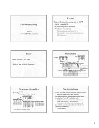
1. Review
Data warehousing: integrating data for OLAP
Data Warehousing • OLAP versus OLTP
• Warehousing versus mediation
• Warehouse maintenance
CPS 216 – Warehouse data as materialized views
– Recomputation versus incremental maintenance
Advanced Database Systems
– Self-maintenance
2
Today Star schema Dimension table
Dimension table Store SID city
Product PID name cost s1 Durham
p1 beer 10 s2 Chapel Hill
• Star, snowflake, and cube p2 diaper 16 s3
…
RTP
…
… … …
Sale OID date CID PID SID qty price Fact table
• ROLAP and MOLAP algorithms 100 11/23/2001 c3 p1 s1 1 12 • Big
102 12/12/2001 c3 p2 s1 2 17 • Constantly growing
105 12/24/2001 c5 p1 s3 5 13 • Stores measures
… … … … … … … (often aggregated in
queries)
Customer CID name address city Dimension table
c3 Amy 100 Main St. Durham • Small
c4 Ben 102 Main St. Durham • Updated infrequently
c5 Carl 800 Eighth St. Durham
… … … …
3 4
Dimension hierarchies Star join indexes
Brand
Product • Queries frequently join fact table with dimension tables
Product type Product category » Materialize the join result to speed up queries
brandID name • For each combination of dimension attribute values,
b1 Huggies
b2 Budwiser store the list of tuple ID’s in the fact table
PID brandID typeID … … – Brand name, store city, customer city → sales records;
p1 b1 t1
p2 b2 t2 typeID name catID catID name Product type, store city → sales records; etc.
p3 b1 t4 t1 diaper cat7 cat7 babies – Conceptually, multi-attribute indexes on the join result
… … … t2 beer cat9 cat9 beverages
t3 juice cat9 … … • One index to support each combination of selection
…
t4 pacifier
…
cat7
…
conditions on attributes?
– Too many indexes!
+ star schema = snowflake schema
5 6
1

2. Bitmap join indexes Data cube
» O’Neil & Quass, SIGMOD 1997 Simplified schema: Sale(CID, PID, SID, qty)
Product
• Bitmap and projection indexes for each
dimension attribute (c5, p1, s3) = 5
– Value of the dimension attribute ↔ tuple ID’s in the (c3, p2, s1) = 2
fact table Store
p2 s3
• To process an arbitrary combination of selection (c3, p1, s1) = 1 (c5, p1, s1) = 3
conditions, use bitmap indexes s2
– Bitmaps can be combined efficiently p1
s1
• To retrieve attribute values for output, use
projection indexes ALL c3 c4 c5
Customer
7 8
Completing the cube (slide 1) Completing the cube (slide 2)
Total quantity of sales for each product in each store Total quantity of sales for each product
SELECT SUM(qty) FROM Sale SELECT SUM(qty) FROM Sale GROUP BY PID;
Product Product
GROUP BY PID, SID;
(c5, p1, s3) = 5 (c5, p1, s3) = 5
(ALL, p1, s3) = 5 (ALL, p1, s3) = 5
(ALL, p2, s1) = 2 (c3, p2, s1) = 2 (ALL, p2, s1) = 2 (c3, p2, s1) = 2
Store (ALL, p2, ALL) Store
p2 (ALL, p1, s1) = 4 s3 =2 p2 (ALL, p1, s1) = 4 s3
(c3, p1, s1) = 1 (c5, p1, s1) = 3 (c3, p1, s1) = 1 (c5, p1, s1) = 3
s2 s2
(ALL, p1, ALL)
p1 =9 p1
s1 Project all points onto Product-Store plane s1 Further project points onto Product axis
Customer Customer
ALL c3 c4 c5 ALL c3 c4 c5
9 10
Completing the cube (slide 3) CUBE operator
Total quantity of sales
» Gray et al., ICDE 1996
SELECT SUM(qty) FROM Sale;
Product
• Sale(CID, PID, SID, qty)
(c5, p1, s3) = 5
(ALL, p1, s3) = 5 • Proposed SQL extension:
(ALL, p2, s1) = 2 (c3, p2, s1) = 2 SELECT SUM(qty) FROM Sale
(ALL, p2, ALL) Store GROUP BY CUBE CID, PID, SID;
=2 p2 (ALL, p1, s1) = 4 s3
(c3, p1, s1) = 1 (c5, p1, s1) = 3 • Output contains:
s2 – Normal groups produced by GROUP BY
(ALL, p1, ALL)
=9 p1 • (c1, p1, s1, sum), (c1, p2, s3, sum), etc.
s1 Further project points onto the origin
– Groups with one or more ALL’s
• (ALL, p1, s1, sum), (c2, ALL, ALL, sum), (ALL, ALL, ALL, sum), etc.
Customer
ALL c3 c4 c5 • Can you write a CUBE query using only GROUP BY’s?
(ALL, ALL, ALL) = 11 11 12
2

3. ROLLUP operator Computing GROUP BY
• Sometimes CUBE is too much • ROLAP (Relational OLAP)
– (…, state, city, street, …, age, DOB, …)
– Use standard relational engine
– CUBE state, city, street returns meaningless groups
• (ALL, ALL, ’Main Street’): sales on any Main Street? – Sorting and clustering
– CUBE age, DOB returns useless groups – Using indexes
• (ALL, DOB): DOB functionally determines age!
– Automatic summary tables
• Proposed SQL extension:
GROUP BY ROLLUP state, city, street; • MOLAP (Multidimensional OLAP)
• Output contains groups with ALL’s only as suffix – Use a sparse multidimensional array
– (’NC’, ’Durham’, ’Main Street’), (’NC’, ’Durham’, ALL),
(’NC’, ALL, ALL), (ALL, ALL, ALL)
– But not (ALL, ALL, ’Main Street’) or (ALL, ’Durham’, ALL)
13 14
Sorting and clustering More on sort order
• Sort (or cluster, e.g., using hashing) tuples • Sort by the order in which GROUP BY attributes
according to GROUP BY attributes appear?
– Tuples in the same group are processed together – Not necessary; e.g., GROUP BY PID, SID can be
– Only one intermediate aggregate result needs to be processed just as efficiently by sorting on SID, PID
kept—low memory requirement • Sort by the order in which GROUP BY ROLLUP
• What if GROUP BY attributes ≠ sort attributes? attributes appear?
– Still fine if GROUP BY attributes form a prefix of the – Useful; e.g., GROUP BY ROLLUP state, city, street
sort order can be processed efficiently by sorting on state, city,
– Otherwise, need to keep intermediate aggregate street, but not by sorting on street, city, state
results around 15 16
Using bitmap join indexes Automatic summary tables
» O’Neil & Quass, SIGMOD 1997 • Computing GROUP BY aggregates is expensive
• Use the bitmap join indexes on GB1, GB2, …, GBk • OLAP queries perform GROUP BY all the time
• For each value v1 of GB1 in order:
For each value v2 of GB2 in order: …
For each value vk of GBk in order: • Idea: precompute and store the aggregates!
Intersect bitmaps to locate tuples; » Automatic summary tables
Retrieve their measures; – Maintained automatically as base data changes
Calculate aggregate for group (v1, v2, …, vk);
– Just another index/materialized view
• Helps if data is sorted by GB1, GB2, …, GBk
– So measures in the same group are clustered
17 18
3

4. Aggregation view lattice Selecting views to materialize
GROUP BY
CID, PID, SID
• Factors in deciding what to materialize
– What is its storage cost?
– What is its update cost?
GROUP BY GROUP BY GROUP BY
CID, PID CID, SID PID, SID – Which queries can benefit from it?
– How much can a query benefit from it?
GROUP BY GROUP BY GROUP BY • Example
CID PID SID – GROUP BY ∅ is small, but not useful to most queries
– GROUP BY CID, PID, SID is useful to any query, but too
A child can be large to be beneficial
GROUP BY ∅
computed from any parent » Harinarayan et al., SIGMOD 1996; Gupta & Mumick,
ICDE 1999
19 20
Interlude: TPC-D, -H, and -R From tables to arrays
• TPC-D: standard OLAP benchmark until 1999 » Zhao et al., SIGMOD 1997
– With aggressive use of precomputation techniques • “Chunk” an n-dimensional cube into n-
(materialized views, automatic summary tables), dimensional subcubes
vendors were able to “cheat” and achieve amazing
– For a dense chunk (>40% full), store it as is
performance
– For a sparse chunk (<40% full), compress it using
• Now, TPC-D has been replaced by <coordinate, value> pairs
– TPC-H: ad hoc OLAP queries
• To convert a table into chunks
• Cannot use materialized views
– Pass 1: Partition table into memory-size partitions,
– TPC-R: business-reporting OLAP queries
each of which contains a number of chunks
• Can use materialized views
– Pass 2: Read partitions back in one at a time, and
» http://www.tpc.org/ 21 chunk each partition in memory 22
Dimension order Basic array cubing
GROUP BY B, C
Memory required:
61 62 63 64 61 62 63 64
45 46 47 48 1 chunk 45 46 47 48
(could be more) ☻
29 30 31 32 29 30 31 32 ☻
Dimension B
Dimension B
☻
60 60 ☻ ☻
13 14 15 16 44 13 14 15 16 44 ☻
28 28 ☻
56 56 ☻ ☻
9 10 11 12 40 9 10 11 12 40 ☻
24 24 ☻
52 Dimension order: 52 ☻ ☻
5 6 7 8 36 A, B, C 5 6 7 8 36 ☻
20 C 20 C ☻
n = Sort order: n
sio sio ☻
1 2 3 4 en C, B, A 1 2 3 4 en
D im D im
23 24
Dimension A Dimension A
4

5. Minimal spanning tree Multiway array cubing
GROUP BY
• Recall the aggregation A, B, C 100 • Goal: compute all 61 62 63 64
aggregates at the 45 46 47 48
lattice same time in a single 29 30 31 32
Dimension B
• MST of the lattice: GROUP BY GROUP BY GROUP BY pass over the array,
A, B 20 A, C 10 B, C 50 60
parent is always using minimum 44
13 14 15 16
amount of memory 28
chosen to be the one GROUP BY GROUP BY GROUP BY 56
• GROUP BY B, C 40
with minimum size A2 B 10 C5 requires 1 chunk
9 10 11 12
24
52
• Compute each node • GROUP BY A, C 36
5 6 7 8
from its parent in the GROUP BY ∅ 1 requires 4 chunks 20 C
n
MST • GROUP BY A, B sio
1 2 3 4 en
requires 16 chunks i m
25 D 26
Dimension A
Memory requirement Minimum-memory spanning tree
• Dimension order is D1, D2, …, Dn • MMST of the aggregation lattice
• Aggregate to compute projects out Dp (i.e., – Parent is always chosen to be the one that makes the
GROUP BY D1, …, Dp – 1, Dp + 1, …, Dn) child require the minimum memory to compute
– Note that results are produced in dimension order too,
• The memory required is roughly
so computation of the entire MMST can be pipelined
| D1 | · | D1 | · … · | Dp – 1 | chunks
– Where | Di | denotes the number of chunks along Di
• Choose an optimal dimension order to minimize
the total amount of memory required by MMST
» It is harder to aggregate away dimensions that
– It turns out that this optimal order is D1, D2, …, Dn,
come later in the dimension order where | D1 | ≤ | D2 | ≤ … ≤ | Dn |
27 28
ROLAP versus MOLAP Next time
• Multiway array cubing algorithm (MOLAP) beats
sorting-based ROLAP algorithms
– Compressed array representation is more compact
than table representation
– Sorting-based ROLAP spends too much time on Data mining
comparing and copying
– In MOLAP, order is implied by the array positions
» An alternative ROLAP techinque
– Convert table to array
– Do MOLAP processing
– Dump the result cube to a table 29 30
5