Keystone XL Pipeline- Market Analysis

Final Supplemental Environmental Impact Statement Chapter 1
Keystone XL Project Introduction
1.4-1
1.4 MARKET ANALYSIS
1.4.1 Introduction and Executive Summary
1.4.1.1 Introduction
This section examines petroleum markets, analyzes how they would be affected by the proposed Project, and assesses whether conclusions from previous market analyses should be altered in light of recent developments. It builds upon and updates the Final Environmental Impact Statement (EIS) published on August 26, 2011, and the Draft Supplemental EIS published on March 1, 2013.
The scope and content of the market analysis that was conducted for the Supplemental EIS were informed by public and interagency comments and new information that was not previously available. Among the notable updates to this analysis are revised modeling to incorporate evolving market conditions, more extensive information on the logistics and economics of crude by rail, and a more detailed analysis of supply costs to inform conclusions about production implications.
The updated market analysis in the Supplemental EIS, similar to the market analysis sections in the 2011 Final EIS and Draft Supplemental EIS concludes that the proposed Project is unlikely to significantly affect the rate of extraction in oil sands areas (based on expected oil prices, oil-sands supply costs, transport costs, and supply-demand scenarios). The Department conducted this analysis, drawing on a wide variety of data and leveraging external expertise. The analysis reflects inputs from other U.S. government agencies and was reviewed through an interagency process.
1.4.1.2 Methodological Overview
The subsections of this analysis examine individual market issues relevant to the proposed Project, which are then integrated to draw conclusions about its potential impact on oil sands production. Section 1.4.2, Oil Market Conditions, provides context on the global oil market, North American upstream and downstream oil industries, supply costs, and recent market developments. Section 1.4.3, Crude Oil Transportation, describes current, planned, or potential midstream crude oil transportation infrastructure, particularly pipelines and rail, which could affect crude oil movements. Section 1.4.4, Updated Modeling, describes key findings from external modeling to indicate how oil trade, refining activities, and price differentials might respond to selected supply-demand and pipeline scenarios.
Conclusions about production impacts of the proposed Project are developed in Section 1.4.5, Conclusions. First, prices from the model results were compared to the long-term supply costs of representative oil sands projects. Second, the difference between modeled prices and oil sands supply costs was examined to approximate how far benchmark oil prices might have to fall before selected oil sands projects would become uneconomic. Third, current and potential transportation options between western Canada and the U.S. Gulf Coast were explored to assess how modeled transportation costs, which affect the prices received by oil sands producers, could vary by mode. The results of these analytical approaches were combined in Section 1.4.5.4, Implications for Production, to draw general conclusions about the production impacts of the proposed Project under various conditions.

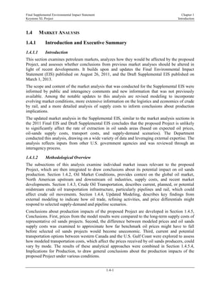
1.4-2
1.4.1.3 Summary of Analysis
The 2011 Final EIS was developed contemporaneously with the start of strong growth in domestic light crude oil supply from tight oil formations. Domestic production of crude oil has increased significantly, from approximately 5.5 million barrels per day (bpd) in 2010 to 6.5 million bpd in 2012 and 7.5 million bpd by mid-2013. Rising domestic crude production is predominantly light crude, and it has replaced foreign imports of light crude oil. However, the demand persists for imported heavy crude oil by U.S. refineries optimized to process heavy crude slates. Meanwhile, Canadian production of bitumen from the oil sands continues to grow, the vast majority of which is currently exported to the United States to be processed by U.S. refineries. North American production growth and logistics constraints have contributed to significant discounts on the price of landlocked crude and led to growing volumes of crude shipped by rail in the United States and, more recently, Canada.
The Draft Supplemental EIS (2013) and Final EIS (2011) discussed the transportation of Canadian crude by rail as a future possibility. Due to market developments since then, this Final Supplemental EIS notes that the transportation of Canadian crude by rail is already occurring in substantial volumes. It is estimated that approximately 180,000 bpd of Canadian crude oil already travel by rail (see Figure 1.4.1-1).
Source: Statistics Canada 2013, U.S. Department of Transportation Bureau of Transportation Statistics 2013, Peters and Co. 2013, IHS Cambridge Energy Research Associates, Inc. (IHS CERA) 2013, and company information.
Figure 1.4.1-1 Estimated Crude Oil Transported by Rail from WCSB, bpd

1.4-3
The industry has been making significant investments in increasing rail transport capacity for crude oil out of the Western Canadian Sedimentary Basin (WCSB). Figure 1.4.1-2 illustrates the increase in rail loading and unloading terminals between 2010 and 2013. Rail-loading facilities in the WCSB are estimated to have a capacity of approximately 700,000 bpd of crude oil, and by the end of 2014, this will likely increase to more than 1.1 million bpd. Most of this capacity (approximately 900,000 to 1 million bpd) is in areas that produce primarily heavy crude oil (both conventional and oil sands), or is being connected by pipelines to those areas.
Various uncertainties underlie the projections upon which the Supplemental EIS partially relies. In recognition of the uncertainty of future market conditions, the analysis included updated modeling about the sensitivity of the market to some of these elements.
Updated information on rail transportation and oil market trends, particularly rising U.S. oil production, was incorporated in oil market modeling. This modeling was developed in response to comments received on the Draft Supplemental EIS. To help account for key uncertainties about oil production, consumption, and transportation, the modeling examined 16 different scenarios that combine various supply-demand assumptions and pipeline constraints. Modeled cases test supply and demand projections based on the official energy forecasts of the independent U.S. Energy Information Administration’s (EIA’s) 2013 Annual Energy Outlook (AEO) that correspond to uncertainties raised in public comments, including potential higher- than-expected U.S. supply, lower-than-expected U.S. demand, and higher-than-expected oil production in Latin America.
The supply-demand cases were paired with four pipeline configuration scenarios: an unconstrained scenario, which allows pipelines to be built without restrictions; a scenario in which no new cross-border pipeline capacity to U.S. markets is permitted but pipelines from the WSCB to Canada’s east and west coasts are built; a scenario where new cross-border capacity between the United States and Canada is permitted but Canadian authorities do not permit new east-west pipelines; and a constrained scenario that assumes no new or expanded pipelines carrying WCSB crude are built in any direction.
Updated model results indicated that cross-border pipeline constraints have a limited impact on crude flows and prices. If additional east-west pipelines were built to the Canadian coasts, such pipelines would be heavily utilized to export oil sands crude due to relatively low shipping costs to reach growing Asian markets. If new east-west and cross-border pipelines were both completely constrained, oil sands crude could reach U.S. and Canadian refineries by rail. Varying pipeline availability has little impact on the prices U.S. consumers pay for refined products such as gasoline or for heavy crude demand in the Gulf Coast. When this demand is not met by heavy Canadian supplies, it is met by heavy crude from Latin America and the Middle East.

1.4-4
-Page Intentionally Left Blank-

1.4-5
Source: Esri 2013. Sources for all facilities are presented in Appendix C, Supplemental Information to Market Analysis. Note: These estimates do not include a facility being constructed in Edmonton, Alberta, with a design capacity of 250,000 bpd (100,000 bpd expected to be operational by the end of 2014) that was announced immediately before the Final Supplemental EIS was completed.
Figure 1.4.1-2 Crude by Train Loading and Off-Loading Facilities in 2010 (top map) and 2013 (bottom map) December 2010
December 2013

1.4-6
-Page Intentionally Left Blank-

1.4-7
Conclusions about the potential effects of pipeline constraints on production levels were informed by comparing modeled oil prices to the prices that would be required to support expected levels of oil sands capacity growth. Figure 1.4.1-3 illustrates existing oil sands capacity, the estimated supply costs of announced capacity, and the capacity growth that will be required to meet EIA and Canadian Association of Petroleum Producers (CAPP) production projections. Projected prices generally exceed supply costs for the projects responsible for future oil sands production growth. Modeling results indicate that severe pipeline constraints reduce the prices received by bitumen producers by up to $8 per barrel, but not enough to curtail most oil sands growth plans or to shut in existing production (based on expected oil prices, oil-sands supply costs, transport costs, and supply-demand scenarios). These conclusions are based on conservative assumptions about rail costs, which likely overstate the cost penalty producers pay for shipping by rail if more economical methods currently under consideration to ship bitumen by rail are utilized.
Source: EIA 2013a, CAPP 2013a, Oil Sands Developers Group (OSDG) 2013, internal analysis Notes: WTI = West Texas Intermediate, $/bbl = dollars per barrel
Figure 1.4.1-3 Oil Sands Supply Costs (WTI-Equivalent $/bbl), Project Capacity, and Production Projections

1.4-8
Several analysts and financial institutions have stated that denying the proposed Project would have significant impacts on oil sands production. To the extent that other assessments appear to differ from the analysis in this report, they typically do so because they have different focuses, near-term time scales, production expectations, and/or include less detailed data and analysis about rail than this report. While short-term physical transportation constraints introduce uncertainty to industry outlooks over the next decade, new data and analysis in the market analysis section indicate that rail will likely be able to accommodate new production if new pipelines are delayed or not constructed.
Over the long term, lower-than-expected oil prices could affect the outlook for oil sands production, and in certain scenarios higher transportation costs resulting from pipeline constraints could exacerbate the impacts of low prices. The primary assumptions required to create conditions under which production growth would slow due to transportation constraints include: that prices persist below current or most projected levels in the long run; and all new and expanded Canadian and cross-border pipeline capacity, beyond just the proposed Project, is not constructed.
Above approximately $75 per barrel (West Texas Intermediate [WTI]-equivalent), revenues to oil sands producers are likely to remain above the long-run supply costs of most projects responsible for expected levels of oil sands production growth. Transport penalties could reduce the returns to producers and, as with any increase in supply costs, potentially affect investment decisions about individual projects on the margins. However, at these prices, enough relatively low-cost in situ projects are under development that baseline production projections would likely be met even with constraints on new pipeline capacity. Oil sands production is expected to be most sensitive to increased transport costs in a range of prices around $65 to 75 per barrel. Assuming prices fell in this range, higher transportation costs could have a substantial impact on oil sands production levels—possibly in excess of the capacity of the proposed Project—because many in situ projects are estimated to break even around these levels. Prices below this range would challenge the supply costs of many projects, regardless of pipeline constraints, but higher transport costs could further curtail production.
Oil prices are volatile, particularly over the short term, and long-term trends, which drive investment decisions, are difficult to predict. Specific supply cost thresholds, Canadian production growth forecasts, and the amount of new capacity needed to meet them are uncertain. As a result, the price threshold above which pipeline constraints are likely to have a limited impact on future production levels could change if supply costs or production expectations prove different than estimated in this analysis.
The dominant drivers of oil sands development are more global than any single infrastructural project. Oil sands production and investment could slow or accelerate depending on oil price trends, regulations, and technological developments, but the potential effects of those factors on the industry’s rate of expansion should not be conflated with the more limited effects of individual pipelines.

1.4-9
1.4.1.4 Previous Analysis
The assessment of the potential market impact of the previously proposed Keystone XL Project was released in the August 26, 2011, Final EIS document. That assessment of the petroleum market drew on several studies, including one commissioned by the U.S. Department of Energy (USDOE) Office of Policy and International Affairs. The USDOE contracted with EnSys Energy and Systems, Inc. (EnSys) to develop a study of different North American crude oil pipeline scenarios through 2030 using EnSys’s World Oil Refining Logistics & Demand (WORLD) model.(Footnote 1).
1 EnSys’s WORLD model provides an integrated analysis and projection of the global petroleum industry that encompasses total liquids, captures the effects of developments, changes, and interactions between regions, and projects the economics and activities of refining crude oils and products. WORLD has been used for DOE’s Office of Strategic Petroleum Reserve since 1987, and has been applied in analyses for many organizations, including the EIA, U.S. Environmental Protection Agency, the American Petroleum Institute (API), the World Bank, the Organization of the Petroleum Exporting Countries (OPEC) Secretariat, the International Maritime Organization, Bloomberg, and major and specialty oil and chemical companies. The conclusions included the following:
•
There was commercial demand for WCSB heavy crude oil in the Gulf Coast. The demand identified by the EnSys 2010 Assessment was sufficiently high that were a permit for the Keystone XL pipeline, as then proposed, denied, the market would likely respond by adding broadly comparable transport capacity over time. The EnSys 2010 Assessment forecasted that the demand for WCSB heavy crude from the oil sands would be such that irrespective of whether a permit for the Keystone XL pipeline, as then proposed, was granted, transport capacity in excess of the Keystone XL pipeline would likely be built.
•
In a situation in which the industry and market react based on normal commercial incentives, neither the production rate in the oil sands nor refining activities in the Gulf Coast would change substantially based on whether Keystone XL, as then proposed, was built.
•
The 2010 EnSys report found the production rate in the oil sands was only substantially reduced in scenarios that assumed all pipeline transport capacity was frozen at 2010 levels through 2030. The scenario also assumed that incremental non-pipeline transport capacity (such as rail or tanker) was not available. The EnSys 2010 report concluded that a No Expansion scenario had a low probability of occurring. Nonetheless, to better assess the No Expansion scenario analyzed by EnSys in 2010, the Department and the USDOE commissioned EnSys to further examine the likelihood of the No Expansion scenario, including assessing in greater detail the potential of non-pipeline transportation of crude oil. In the 2011 No Expansion Update, EnSys concluded that even if there were no new pipelines added beyond those existing in 2010, rail supported by barge and tanker, as well as expansions to refining/upgrading in Canada, could accommodate projected oil sands production.
Other sources consulted in preparing the 2011 Final EIS included input from experts at the USDOE, information from industry associations (CAPP) and private consulting companies such as Purvin & Gertz, IHS Cambridge Energy Research Associates, Inc. (IHS CERA), Hart Energy, and ICF International, as well as the numerous comments received from the public. Taking account of all of the relevant information, the 2011 Final EIS concluded that the proposed Project is unlikely to significantly affect the rate of extraction in the oil sands or in U.S. refining

1.4-10
activities. The Final EIS nonetheless, as a matter of policy, included information about the environmental impacts associated with extraction of crude oil in the oil sands, particularly an extensive analysis of the fact that on a lifecycle basis, transportation fuels produced from oil sands crudes emit more greenhouse gases than most conventional crude oils.(Footnote 2).
2 This information and analysis is updated in this Final Supplemental EIS in Section 4.14, Greenhouse Gases and Climate Change.
The March 1, 2013, Draft Supplemental EIS examined petroleum market changes since the 2011 Final EIS was issued and whether these changes alter the conclusion of the 2011 Final EIS. It took into account increases for domestic oil production, decreases in expected demand, and changes in infrastructure, particularly the increase in oil transport by rail and found the following:
•
While the increase in U.S. production of crude oil and the reduced U.S. demand for transportation fuels will likely reduce the demand for total U.S. crude oil imports, it is unlikely to reduce demand for heavy sour crude at Gulf Coast refineries. Additionally, as was projected in the 2011 Final EIS, the midstream industry is showing it is capable of developing alternative capacity to move WCSB (and Bakken and Midcontinent) crudes to markets in the event the proposed Project is not built. Specifically, alternative pipeline capacity is being developed that would support WCSB crude oil movements to U.S. and foreign markets, and also that rail was available to transport large volumes of crude oil to East, West, and Gulf Coast markets as a viable alternative to pipelines. In addition, projected crude oil prices are sufficient to support production of oil sands (and U.S. tight oil(Footnote 3).
3 Tight oil or shale oil refers to oil found in low-permeability and low-porosity reservoirs, typically shale. Bakken crude from the Williston Basin in North Dakota and Montana is considered tight oil. The technology of extracting crude oil from tight rock formations has only recently been exploited at scale, but produces and supplies large quantities of crude oil into the domestic market. ). Rail and supporting non-pipeline modes should be capable, as was projected in 2011, of providing the capacity needed to transport all incremental western Canadian and Bakken crude oil production to markets if there were no additional pipeline projects approved.
•
Approval or denial of any one crude oil transport project, including the proposed Project, remains unlikely to significantly impact the rate of extraction in the oil sands, or the continued demand for heavy crude oil at refineries in the United States. Limitations on pipeline transport would force more crude oil to be transported via other modes of transportation, such as rail, which would probably (but not certainly) be more expensive. Longer term limitations also depend upon whether pipeline projects that are located exclusively in Canada proceed (such as the proposed Northern Gateway, the Trans Mountain expansion, and the TransCanada Corporation [TransCanada] proposal to ship crude oil east to Ontario on a converted natural gas pipeline). The Draft Supplemental EIS estimated that if all such pipeline capacity were restricted in the medium-to-long term, the incremental increase in cost of the non-pipeline transport options could result in a decrease in production from the oil sands, perhaps 90,000 to 210,000 bpd (approximately 2 to 4 percent) by 2030. The Draft Supplemental EIS also estimated that if the proposed Project were denied but other proposed new and expanded pipelines go forward, the incremental decrease in production could be approximately 20,000 to 30,000 bpd (from 0.4 to 0.6 percent of total WCSB production) by 2030.

1.4-11
As in 2011, the analysis in the Draft Supplemental EIS again was informed by consultation with experts from USDOE and information from industry associations such as CAPP and private consulting companies such as EnSys, Hart Energy, and ICF International. The Draft Supplemental EIS also relied on a January 2013 memorandum from the Administrator of the EIA (see Appendix C, Supplemental Information to Market Analysis) that analyzed some of the key issues also presented in this section.
In response to public and agency comments on the Draft Supplemental EIS, this Final Supplemental EIS has updated and expanded its analysis, including on oil sands supply costs, rail transport costs, the EnSys modeling, and expected impacts on production.
1.4.2 Oil Market Conditions(Footnote 4).
4 This section describes oil market conditions using historical data and projections available as of November 15, 2013. The Early Release of the Reference Case from the 2014 AEO occurred after this section was prepared. AEO2014 Reference Case projections update the AEO2013 projections referenced here, but remain substantially similar with regard to the issues considered. AEO2014 Reference Case projections generally fall within the range of the AEO2013 cases assessed in this report. The full version of the AEO2014 will not be released until Spring 2014.
1.4.2.1 Global Oil Market Context
The United States is part of a globally integrated oil market. Crude oil makes up roughly 75 million bpd out of a roughly 90 million bpd total oil market.(Footnote 5).
5 Global crude oil supply in 2012 was roughly 75 million bpd according to the International Energy Agency (IEA) Monthly Oil Market Report (IEA 2012a). That crude must be refined into fuels, which can then be consumed as is discussed below. A volumetric increase that occurs as crudes are broken down into fuels means that 75 million barrels of crude corresponds with a slightly greater amount of liquid fuels. Apart from crude-based fuels, other liquid fuels that help meet global oil demand include natural gas liquids, biofuels, and coal or gas transformed into liquid fuels. More than 60 percent of the world’s oil is traded internationally.(Footnote 6).
6 Globally traded oil amounted to 62 percent of global consumption in 2012, according to the BP Statistical Review of World Energy (BP 2013). In 2012, the United States accounted for 20 percent of global oil consumption. Expectations for oil market growth vary, with many projecting that global consumption will grow to 100 million bpd or more by 2035.
Supply and demand trends will drive long-term prices in this global market. Due to the integrated nature of the global oil market, oil prices tend to move together. Nonetheless, benchmark prices may differ due to quality discounts and transportation costs. The supply and demand for oil are relatively price inelastic (unresponsive to price changes), at least in the short run. Exogenous shocks to demand and/or supply will therefore translate into relatively large price changes.
The United States and other members of the Organization for Economic Cooperation and Development (OECD), a group of the world’s advanced economies, consumed just over half of the world’s liquid fuels in 2012.(Footnote 7).
7 These global trends and those discussed below reflect widely held expectations, including in the EIA AEO and International Energy Outlook, the IEA World Energy Outlook (WEO), and other long-term oil market projections. OECD consumption is not anticipated to grow substantially, if at all, over the foreseeable future due to efficiency policies, modest economic growth driven by non-industrial sectors, and generally because many of the energy-intensive needs of OECD consumers are already being met.

1.4-12
Most oil consumption growth going forward is likely to come from rapid economic development in non-OECD regions. Key economies driving energy demand growth include China, India, and the countries of the Middle East.
Supply to meet this rising demand will come from a diverse set of resources around the world. Some of the largest sources of additional supply through 2035, according to many analysts, include unconventional oil resources—such as those trapped in U.S. shale or the offshore subsalt in Brazil—as well as the large conventional oil resources of the Middle East. Many analysts also expect substantial growth in Canada’s oil sands. The prospects for this are discussed more fully throughout this document.
1.4.2.2 U.S. Oil Market Overview
The subsection provides context and background on U.S. oil market conditions as of 2013. In general, U.S. domestic crude oil and related liquid fuels production has increased in recent years. Consumption fell from 2007 to 2009 and has averaged between 18.5 to 19.2 million bpd since then. The United States consumed 18.6 million bpd of liquid fuels in 2012, primarily fuels refined from crude oil (see Table 1.4.1). This demand was met through a combination of domestic crude production, other domestic liquid fuels production, crude imports, and imports of non-crude liquids (including refined products). Of the imported crude, 2.4 million bpd came from Canada.
For data collection and analysis, the 50 U.S. states and the District of Columbia are divided into five regions called Petroleum Administration for Defense Districts (PADDs) (see Figure 1.4.2-1).(Footnote 8).
8 The origin of PADDs dates from World War II when it was necessary to allocate domestic petroleum supplies. The boundaries between the different PADDs do not reflect either a regulatory or a business requirement, but provide the EIA with a mechanism to consistently report the key attributes of the petroleum industry (inventory, crude processing levels, prices, consumption, etc.) over various time periods. The supply and refining profiles of the PADDs differ significantly. For example, PADD 3 and PADD 1 both import significant amounts of crude oil. PADD 3 imports a wider variety of crude oils, including over 2 million bpd of heavy crude oil, whereas PADD 1 imports are almost entirely of light and medium crude oils. Refiners in different PADDs largely serve the market for transportation fuels and other products in that PADD, but there are inter-PADD transfers and refiners in the different PADDs are in competition with one another. In particular, PADD 3 refiners ship refined products to both PADD 1 and PADD 2. Additional information about the PADDs, including their refining and supply profiles, is included in Section 2.0 of Appendix C, Supplemental Information to Market Analysis.

1.4-13
Table 1.4-1 U.S. Liquid Fuel Supply-Demand Balance, 2012 (million bpd)
U.S. Liquid Fuels Consumption
18.6
Gasoline
8.7
Distillate Fuel Oil/Diesel
3.7
Other
6.1
Crude Oil Supply
14.9
Domestic crude production
6.5
Net crude imports
8.4
Gross Crude Imports
8.5
from Canada
2.4
from Other
6.1
Exports to Canada
-0.1
Other Supply
3.4
Natural Gas Liquids Production
2.4
Refinery Processing Gain(Footnote a).
1.1
Renewables and Oxygenates Production
1.0
Net Petroleum Product Imports
-1.0
Gross Imports
2.1
Imports from Canada
0.5
Imports from Others
1.6
Gross Exports
-3.1
Exports to Canada
-0.3
Exports to Others
-2.8
Source: EIA 2013a. Notes: May not sum due to rounding. Inventory withdrawal and adjustments amounting to 0.3 million bpd are not listed. Exports are listed as negative values. U.S. origin crude is only exported to Canada. (Footnote a). Refinery processing gain is the volumetric amount by which total output (refined products) is greater than input (crude oil) for a given period of time. According to EIA’s definition, “this difference is due to the processing of crude oil into products which, in total, have a lower specific gravity than the crude oil processed”.
Source: EIA 2012b
Figure 1.4.2-1 Petroleum Administration for Defense Districts (PADD) Locations

1.4-14
1.4.2.3 U.S. Crude Oil Production
The 2011 Final EIS was developed contemporaneously with the beginnings of strong growth in domestic light crude oil supply from shale, or tight oil, formations.(Footnote 9). U.S. tight oil sources include the Bakken in the Williston Basin of North Dakota and Montana; the Eagle Ford in South Texas; the Permian in West Texas and New Mexico; the Mississippian Lime in Oklahoma and Kansas; the Tuscaloosa Marine Shale in Louisiana; the Monterey and Kreyenhagen in California; the Avalon, Bone Springs, and Wolfberry in the Permian Basin of Texas and New Mexico; the Niobrara in Colorado and Wyoming; and the Utica shale in Ohio and Pennsylvania. Among these, the Bakken and Eagle Ford have been the main sources of supply growth to date. Domestic production of crude oil has increased significantly, from approximately 5.5 million bpd in 2010 to 6.5 million bpd in 2012 and 7.5 million bpd by mid-2013. In addition to contributing to significant discounts on the price of inland crude because of logistics constraints,(Footnote 10). The discount for PADD 2 crude did not translate to a discount for refined products in PADD 2. The discount for PADD 2 crude was due to infrastructure bottlenecks for crude transport from PADD 2 to PADD 3 and elsewhere. Inter-regional refined products movements kept prices for gasoline and other refined products in PADD 2 in line with their historic relationship with products prices elsewhere in the United States. The resulting widened differential between PADD 2 crude and products prices benefited PADD 2 refiners. See Section 1.4.6.1, Crude Price Differences and Gasoline Prices. there has been a sharp reduction in U.S. imports of crude oil, particularly light sweet crude oil.
Domestic crude production is expected to grow further in the coming years, but there is uncertainty about how high supplies will go and how long they will remain elevated. The 2013 EIA AEO Reference Case projects domestic crude output will peak at 7.5 million bpd in 2019 and then decline to 6 million bpd by 2035 (see Figure 1.4.2-2). EIA’s High Oil and Gas Resources case, which assumes higher recovery rates from tight oil resources, projects crude production rises to 10 million bpd by 2025 and remains at that level through 2035.(Footnote 11).
9
10
11 “In the High Oil and Gas Resources case, resource assumptions are adjusted to give continued increase in domestic crude oil production after 2020, reaching over 10 million barrels per day. This case includes: (1) 100 percent higher EUR [estimated ultimate recovery] per tight oil, tight gas, and shale gas well than in the Reference case and a maximum well spacing of 40 acres, to reflect the possibility that additional layers of low-permeability zones are identified and developed, compared with well spacing that ranges from 20 to 406 acres with an average of 100 acres in the Reference case; (2) kerogen development reaching 135,000 barrels per day in 2025; (3) tight oil development in Alaska increasing the total Alaska TRR [technically recoverable resources] by 1.9 billion barrels; and (4) 50 percent higher technically recoverable undiscovered resources in Alaska and the offshore lower 48 states than in the Reference case. Additionally, a few offshore Alaska fields are assumed to be discovered and thus developed earlier than in the Reference case. Given the higher natural gas resource in this case, the maximum penetration rate for GTL [gas-to-liquids] was increased to 10 percent per year, compared to a rate of 5 percent per year in the Reference case.” (EIA 2013a).

1.4-15
Source: EIA 2013a
Figure 1.4.2-2 AEO Forecasts for Domestic Crude and Condensate Production
Other forecasts also reflect a wide range of expectations. The 2013 International Energy Agency (IEA) World Energy Outlook (WEO) expects U.S. crude oil production to climb until 2025, reaching 8.8 million bpd before falling to 8.6 million bpd by 2035.(footnote 12).
12 Data from IEA analysis for the 2012 WEO. Timur Gould, personal communication, December 5, 2013. Oil industry consultant PIRA Energy Group expects U.S. crude oil production to rise to 11.6 million bpd by 2025 before starting to decline, reaching 11.4 million bpd by 2030.(footnote 13).
13 Victoria Watkins, personal communication, 2013. Investment research firm Sanford C. Bernstein expects crude production to reach 8.1 million bpd in 2019 and then decline to 5.6 million bpd by 2030.(footnote 14).
14 Helin Shiah, personal communication, December 2013.
While expected peak output levels and years vary, most other forecasts—like the Reference Case—expect U.S. production growth to be driven by light, tight oil and to peak between 2019 and 2025 before starting to decline. In contrast, EIA’s High Resource Case projects relatively flat production at elevated levels after 2020. Uncertainty about future technology, geology, development costs, oil prices, policy, and other factors drive differences in expectations.

1.4-16
1.4.2.4 U.S. Oil Consumption
U.S. liquid fuels consumption averaged 18.6 million bpd in 2012, down from a peak of 20.8 million bpd in 2005. As shown in Table 1.4-2, consumption declined across fuels, including gasoline. Economic weakness and efficiency improvements have contributed to the decline.
Table 1.4-2 Fuels Consumption by Product (million bpd)
Product
2005
2010
2012
NGLs and LRGs
2.15
2.27
2.32
Finished Motor Gasoline
9.16
8.99
8.70
Distillate Fuel Oil
4.12
3.80
3.74
Kerosene—Type Jet Fuel
1.68
1.43
1.40
Finished Aviation Gasoline
0.02
0.02
0.01
Residual Fuel Oil
0.92
0.54
0.35
Other Liquids
0.01
0.01
0.08
Source: EIA 2013a
In EIA’s Reference Case (EIA 2013a), consumption is expected to rise to 19.8 million bpd in 2019 and then fall, leveling off at 18.9 million bpd after 2030 (see Figure 1.4.2-3). Divergent trends across fuels would underlie aggregate consumption near today’s levels: A 1.7 million bpd decline in gasoline consumption by 2035 is offset by rising demand for distillate fuel oil (primarily diesel), liquefied petroleum gases, and jet fuel (see Figures 1.4.2-4, 1.4.2-5, and 1.4.2-6). The Reference Case projections reflect improving efficiency, such as the Corporate Average Fuel Economy (CAFE) standards for model years 2012 through 2025, and slowing growth in vehicle miles traveled as a result of demographic changes. For an expanded discussion on efficiency improvements, see Section 2.2, Description of Alternatives.
In its Low/No Net Imports case, where the EIA makes assumptions that lead to lower oil demand,(Footnote 15).
15 “In the Low/No Net Imports case, changes were made to various NEMS [National Energy Modeling System] modeling assumptions that, in comparison with the AEO 2013 reference case, resulted in higher domestic production of crude oil and natural gas, lower domestic liquid fuels demand, and higher domestic production of nonpetroleum liquids. The methodology used to achieve higher domestic crude production is the same as that used in the High Oil and Gas Resource case (described in the “Oil and gas supply cases” section above). Domestic liquid fuels demand was reduced by changes made in the Transportation Demand Module. As described in the “Transportation sector cases” section, this included the use of more optimistic assumptions about improvements in LDV [light-duty vehicle] fuel economy and reductions in LDV technology costs; lower VMT [vehicle miles travelled] due to changes in consumer behavior; an extension of the LDV CAFE standards beyond 2025 at an average annual rate of 1.4 percent through 2040; expanded market availability of LNG [liquified natural gas]/CNG [compressed natural gas] fuels for heavy-duty trucks, rail, and marine; and use of assumptions from the optimistic battery case (EIA 2012a) for electric vehicle battery and drivetrain costs. Within the LFMM [Liquid Fuels Market Module], the assumption for market penetration of biomass pyrolysis oils, CTL [carbon-to-liquids], and BTL [biomass-to-liquids] production was more optimistic. Also, initial assumptions associated with E85 availability and maximum penetration of E15 were set to be more optimistic, such that E85 availability was nearly three times the Reference case level in 2040, and E15 penetration was about 15 percent higher by 2040.” (EIA 2013a). EIA projects a smaller increase in consumption in this decade and then a decline after 2020, with consumption falling to around 17 million bpd by 2035. Most of the difference with the Reference Case is accounted for by lower projected gasoline and distillate fuel oil consumption due in large part to the Low/No Net Imports case assumption that vehicle miles traveled continually decline.

1.4-17
Source: EIA 2013a
Figure 1.4.2-3 AEO Forecasts for U.S. Liquid Fuels Consumption
Source: EIA 2013a
Figure 1.4.2-4 AEO Gasoline/E85 Consumption

Source: EIA 2013a
Figure 1.4.2-5 AEO Diesel Consumption 1.4-18
Source: EIA 2013a Note: Consumption of liquid fuels excluding gasoline, E85, and diesel is higher in the Low/No Imports Case than the Reference Case due primarily to differing assumptions about oil and natural gas production, which contributes to greater use of liquefied petroleum gases.
Figure 1.4.2-6 Other Liquids Fuels Consumption (excluding Gas/E85, and Diesel)

1.4-19
1.4.2.5 U.S. Refining
The petroleum products that make up the vast majority of U.S. and global oil consumption must be processed from crude oil in a refinery. Refineries break crude oil down into its various components, which then are selectively reconfigured into products. In 2012, the United States had 19.0 million bpd of crude distillation capacity, the simplest form of crude refining.(Footnote 16).
16 For data availability reasons, this figure and the data in Table 1.4-3 are based on “barrels per stream day,” which according to EIA is “The maximum number of barrels of input that a distillation facility can process within a 24-hour period when running at full capacity under optimal crude and product slate conditions.” The United States had 17.3 million bpd of atmospheric crude distillation capacity in terms of barrels per calendar day, or the amount of input that a distillation facility can process under usual operating conditions. Crude distillation units (CDU) separate crude oil into fractions. These are then further processed and treated to produce finished fuels, some of which also contain blending components. Some U.S. refineries integrate CDUs with more complex processing units that can upgrade heavier fractions of crude oil coming from the CDU into more valuable fuels. More complex refining capacity such as catalytic cracking and coking units are concentrated in PADD 3 (see Table 1.4-3, Figures 1.4.2-7, and 1.4.2-8 below), which has traditionally imported heavy crude from sources including Venezuela and Mexico.
Cokers are the downstream processing unit necessary to process the heaviest fractions from crude oils, called residuum. The United States has over half of the world’s coking(Footnote 17).
17 Coking is a refinery operation that is used to process heavy crude oil. The process upgrades material into higher value products and produces petroleum coke (EIA 2013b). capacity, and the majority of this capacity is at Gulf Coast refineries (1.6 million bpd capacity in PADD 3 out of 2.85 million bpd nationwide in 2012), according to EIA data.
Refineries build units in configurations and combinations that run optimally with certain kinds of crudes. Lighter crudes, or those with higher American Petroleum Institute (API) gravity(Footnote 18).
18 API gravity is the API’s scale for expressing the gravity or density of crude oil (among other liquids). Water has an API gravity of 10. There is a range of cutoff points that are used to specify heavy crude oil. Generally, an API gravity of around 28 is considered the cutoff for the lightest heavy crude that is suited to processing in a deep conversion refinery, one that usually in the United States has a coker to upgrade the heaviest residuum fractions to light products. Nonetheless, a common cutoff is 25 API and that is what is used in this analysis. For comparison, Brent crude has an API gravity of about 38 and WTI has an API gravity of around 40. Crude oils from shale range from an API gravity of around 38 (Bakken crude) to 45 (Eagle Ford crude). Diluted bitumen, or dilbit, has API gravity of around 20. , yield historically more valuable products, such as gasoline and diesel, with less processing than heavier crudes. Heavier crudes yield relatively more low-value products through distillation, which can then be upgraded to lighter, more valuable products through more complex refining processes described briefly above. As a result of processing costs and/or the value of product yields, heavier crudes trade at a discount to lighter crudes. A refinery can be built to process a heavier slate of crudes depending on what units are built and how they are configured to run together. A refiner can also invest in units which can remove sulfur from oil, allowing a refinery to process higher sulfur crude oils and still produce fuels that meet U.S. sulfur limits. The configuration of a refinery is an integrated system which has some flexibility to alter the types of crudes run with regard to API gravity, sulfur content, and other characteristics. However, large changes in the crude slate require investment in new units and the reconfiguration of existing operations; hence refiners have an incentive to process the crude oil slate for which they are configured.

1.4-20
Table 1.4-3 Refining Charge Capacity by Unit and PADD
(Barrels per Stream Day)
Atmospheric Distillation Capacity(Footnote a).
Vacuum Distillation(Footnote b).
Coking/
Thermal Cracking(Footnote c).
Catalytic Cracking(Footnote d).
Catalytic Reforming(Footnote e).
Hydrotreating/ Desulfurization(Footnote f).
Fuels Solvent Deasphalting(Footnote g).
PADD 1
1,361,700
586,400
81,500
573,500
263,950
1,092,500
22,000
PADD 2
4,063,188
1,703,312
502,276
1,322,501
906,807
3,601,746
17,850
PADD 3
9,664,455
4,781,775
1,608,880
3,169,105
1,845,790
9,030,080
241,400
PADD 4
672,300
240,600
89,300
205,350
133,600
563,660
6,000
PADD 5
3,210,000
1,626,006
595,500
903,300
608,200
2,572,200
80,300
Total
18,971,643
8,938,093
2,877,456
6,173,756
3,758,347
16,860,186
367,550
Source: EIA 2013d (Footnote a).The refining process of separating crude oil components at atmospheric pressure by heating to temperatures of about 600 degrees to 750 degrees Fahrenheit (depending on the nature of the crude oil and desired products) and subsequent condensing of the fractions by cooling. (Footnote b).Distillation under reduced pressure (less the atmospheric), which lowers the boiling temperature of the liquid being distilled. This technique with its relatively low temperatures prevents cracking or decomposition of the charge stock. (Footnote c). Thermal cracking is a refining process in which heat and pressure are used to break down, rearrange, or combine hydrocarbon molecules. Thermal cracking includes gas oil, visbreaking, fluid coking, delayed coking, and other thermal cracking processes. Coking describes a thermal refining processes used to produce fuel gas, gasoline blendstocks, distillates, and petroleum coke from the heavier products of atmospheric and vacuum distillation. This category is primarily coking units with 26,600 bpd of other units included. (Footnote d). The refining process of breaking down the larger, heavier, and more complex hydrocarbon molecules into simpler and lighter molecules. Catalytic cracking is accomplished by the use of a catalytic agent and is an effective process for increasing the yield of gasoline from crude oil. Catalytic cracking processes fresh feeds and recycled feeds. Includes fresh feed and recycle feed. (Footnote e). A refining process using controlled heat and pressure with catalysts to rearrange certain hydrocarbon molecules, thereby converting paraffinic and naphthenic type hydrocarbons (e.g., low octane gasoline boiling range fractions) into petrochemical feedstocks and higher octane stocks suitable for blending into finished gasoline. (Footnote f). A refining process for treating petroleum fractions from atmospheric or vacuum distillation units (e.g., naphthas, middle distillates, reformer feeds, residual fuel oil, and heavy gas oil) and other petroleum (e.g., cat cracked naphtha, coker naphtha, gas oil, etc.) in the presence of catalysts and substantial quantities of hydrogen. Hydrotreating includes desulfurization, removal of substances (e.g., nitrogen compounds) that deactivate catalysts, conversion of olefins to paraffins to reduce gum formation in gasoline, and other processes to upgrade the quality of the fractions. (Footnote g). A refining process for removing asphalt compounds from petroleum fractions, such as reduced crude oil. The recovered stream from this process is used to produce fuel products. Note: Reference to total refining capacity is typically based on atmospheric distillation capacity. Definitions above from the EIA Glossary.

1.4-21
Rest of World (113 Countries) 26% Venezuela 3% Mexico 4% Japan 3% India 4% Brazil 2% China 3% U.S. 55%
Source: Canadian Imperial Bank of Commerce (CIBC) 2012
Figure 1.4.2-7 Distribution of Global Coking Capacity U.S. PADD 13%U.S. PADD 218% U.S. PADD 356% U.S. PADD 43% U.S. PADD 520%
Source: EIA 2013a
Figure 1.4.2-8 Distribution of U.S. Coking Capacity

1.4-22
1.4.2.6 Demand for Heavy Imported Crude
Table 1.4-4 shows heavy crude imports (25 API gravity and below) in the first half of 2013 for Gulf Coast area refiners that are in the immediate anticipated destination market for the proposed Project.(Footnote 19).
19 Includes refineries importing heavy crude in the first half of 2013 between Corpus Christi and Lake Charles (i.e., not the New Orleans refinery sector). This table indicates that there are about 1.4 million bpd of heavy crude imports into refineries along the Gulf Coast area through Lake Charles, Louisiana. Actual heavy crude processing capacity is higher than current levels of heavy crude imports.
Table 1.4-4 Proposed Project Destination Area Refiners Heavy Crude Processing, January to June 2013(Footnote a).
a This table includes all refineries importing heavy crude (<25 API) between Corpus Christi, Texas, and Lake Charles, Louisiana. In the eastern Gulf Coast area (New Orleans and Baton Rouge areas), over the same time period (January to June 2013) there were 17 refineries with combined total refining capacity of 3.01 million bpd, and these refineries imported 513,773 bpd of heavy crude.
Refiner
Heavy Crude Imports (bpd)
Number of Refineries
Top 2 Import Sources of Heavy Crude
Valero Refining Co Texas LP
315,022
3
Mexico, Venezuela
CITGO Petroleum Corp
255,376
2
Venezuela, Angola
Houston Refining LP
192,122
1
Colombia, Venezuela
Phillips 66 Company
175,260
2
Venezuela, Mexico
Deer Park Refining LTD Partnership
144,039
1
Mexico, Venezuela
ExxonMobil Refining & Supply Co
143,133
2
Mexico, Colombia
Motiva Enterprises LLC
80,923
1
Venezuela, Brazil
Total Petrochemicals & Refining USA
73,448
1
Venezuela, Mexico
Marathon Petroleum Co LLC
31,293
2
Kuwait, Mexico
Pasadena Refining Systems Inc.
5,309
1
Angola
Total
1,415,923
16
Source: EIA Refinery Capacity Report (EIA 2013d). Data as of January 1, 2013; EIA Company Level Imports (EIA 2013c). Note: Although Flint Hill Resources LP has a small coker and has imported heavy crude from Brazil from January to June, the coker is currently idling.
Over the last five years, the average quality of crudes processed in U.S. refineries stopped declining, moving up slightly from 30.4 degrees API gravity in 2007 to 31.0 degrees API gravity in 2012 (see Figure 1.4.2-9).
Underlying this is a shift in sourcing for light versus heavy crudes. Rising domestic light crude production has backed out foreign imports of light crude oil. However, refiners optimized for crude slates that use heavy crudes still have demand for heavy crude and continue to meet that demand through imports. Figure 1.4.2-10 shows decreasing volumes of light crude imports while heavy crude imports remain robust. Refiners’ preferences for heavier crudes appear to be enduring despite rising domestic light supplies. This reflects refinery optimization for certain kinds of crudes. Consequently, growing domestic light crude production is backing out (reducing) light imports, and may be blended with heavier crudes to back out medium grade imports.

Source: EIA 2013a
Figure 1.4.2-9 Average Quality of Crude Oil Input to Refineries - 2.0 4.0 6.0 8.0 10.0 12.0200220032004200520062007200820092010201120122013YTD Million Barrels per Day Over 40.035.1 to 40.030.1 to 35.025.1 to 30.020.1 to 25.020.0 or less
Source: EIA 2013a
Figure 1.4.2-10 Average Annual Imports by API Gravity, thousand bpd 1.4-23

1.4-24
As a result, the average quality of crude imports is growing heavier (see Figure 1.4.2-11). The EIA AEO explicitly forecasts that U.S. imports will continue growing heavier on average in its Reference Case.
Source: EIA 2013a
Figure 1.4.2-11 Quality of Domestic and Imported Crude Processed by U.S. Refiners
While EIA does not explicitly forecast the quality of crude imports in other cases, it is likely that the average gravity of imported crude would be even heavier in the High Resource and Low/No Net Imports cases. The High Resource Case projects the United States continues gross crude oil imports of 3.4 million bpd or more through 2035. Because the additional domestic crude supply in the High Resource versus the Reference Case is largely light, tight oil, it is likely that what crude is imported is even heavier on average than in the Reference Case. Even in the Low/No Net Imports case—which is built on top of the domestic production assumptions in the High Resource Case—the United States is expected to continue gross imports of crude at 3.1 million bpd or higher and again it is likely that these trend even heavier than in the Reference Case on average.
The EIA notes, “AEO2013, AEO2012, and AEO2011 all project continued strong demand for heavy sour crudes from Gulf Coast refiners that are optimized to process such oil” (see the EIA January 2013 memo in Appendix C, Supplemental Information to Market Analysis). A main driver for this is that although refiners can be expected to make adjustments in their operations to take advantage of the increased supply of light crudes on the markets, shutting down their heavy crude upgrading units would likely be an inefficient and expensive option. Given the

1.4-25
concentration of upgrading units in PADD 3 and the economic incentives to run heavy crudes given light-heavy oil price differentials, this region will likely remain a key source of heavy crude demand. However, options for refinery reconfiguration were included in the modeling described in Section 1.4.4, Updated Modeling, to test how heavy crude demand might change due to increased supplies of light crude.
1.4.2.7 Oil Trade
U.S. net imports of crude and petroleum product averaged 7.4 million bpd in 2012 (see Table 1.4-5). This is 5.1 million bpd lower than its peak in 2005 due to supply and demand changes described above. These developments have manifested as both a decline in gross imports of crude and petroleum products and an increase in exports of petroleum products.
Table 1.4-5 Gross Imports and Exports of Crude Oil and Petroleum Products (thousand bpd)
Gross Imports
Gross Exports
Net Imports
2005
2010
2012
2005
2010
2012
2005
2010
2012
Crude Oil
10,126
9,213
8,491
32
42
60
10,094
9,171
8,431
Petroleum Products
3,588
2,580
2,105
1,133
2,311
3,124
2,455
269
-1,019
Total
13,714
11,793
10,596
1,165
2,353
3,184
12,549
9,440
7,412
Source: EIA 2013a
Crude Oil Trade
Gross crude oil imports fell from 10.1 million bpd in 2005 to about 8.5 million bpd in 2012. Imports fell in all PADDs except PADD 2, and to a lesser extent PADD 5, where imports from Canada have increased (see Table 1.4-6 and Table 1.4-7).
Table 1.4-6 Crude Imports by Processing PADD (thousand bpd)
2005
2010
2012
PADD 1
1,602
1,093
859
PADD 2
1,516
1,377
1,720
PADD 3
5,650
5,329
4,467
greater than or = 25 API
3,378
2,985
2,285
< 25 API
2,272
2,343
2,194
PADD 4
271
225
234
PADD 5
1,056
1,139
1,145
Total
10,096
9,163
8,424
Source: EIA 2013c (Company Level Imports)

1.4-26
Table 1.4-7 Crude Imports by Port PADD (thousand bpd)
2005
2010
2012
PADD 1
1,602
1,092
854
PADD 2
1,006
1,207
1,726
PADD 3
6,099
5,400
4,385
greater than or = 25 API
3,785
3,149
2,315
< 25 API
2,314
2,251
2,069
PADD 4
332
325
315
PADD 5
1,056
1,139
1,146
Total
10,096
9,163
8,424
Source: EIA 2013c (Company Level Imports)
Rising domestic light crude supplies, the configuration of domestic refineries, and production trends abroad have shaped where U.S. imports come from, as shown in Figure 1.4.2-12. For instance, imports from West Africa, which has traditionally supplied light crude oil to the United States, have been backed out by rising U.S. light crude oil production.
0
2
4
6
8
10
12
2000
2001
2002
2003
2004
2005
2006
2007
2008
2009
2010
2011
2012
Million Barrels per Day
Other non-OPEC
Other OPEC, ex Persian Gulf
Nigeria
Other Persian Gulf
Saudi Arabia
Kuwait
Colombia
Canada
Mexico
Venezuela
Source: EIA 2013a
Figure 1.4.2-12 Gross U.S. Crude Oil Imports by Major Foreign Sources(Footnote 20). 20 The United States primarily imports crude comparable in quality to dilbit from five countries: Canada, Mexico, Venezuela, Colombia, and Kuwait.

1.4-27
Imports from Mexico and Venezuela, traditional heavy oil suppliers, fell during the 2000s as production from those countries declined. EIA’s forecast implies that net oil exports from these countries will continue to decline.(Footnote 21).
21 Though it does not break out individually Mexican and Venezuelan production, consumption, and thus net exports, it aggregates them in ways that the trend is relatively clear. For both production and consumption, Mexico is aggregated with Chile, the other OECD country in Latin America which produces negligible amounts of oil. Production for the grouping falls by 1 million bpd by 2020 to 2 million bpd and remains near that level for the rest of the forecast. Meanwhile consumption for the group grows steadily. Venezuela’s production is grouped with Ecuador, the other OPEC country in Latin American, and the grouping’s production is roughly flat in the range of 2.9 to 3.2 million bpd throughout the forecast. Venezuela’s consumption is more difficult to identify as it is grouped with all of Central and South America except Brazil. That group’s consumption rises from 3.4 to 3.9 million bpd. There is uncertainty about how production levels will develop and both countries are looking to alter the trend, which are explored further in Section 1.4.4, Updated Modeling. However, even if this trend changes, Mexican production is becoming lighter on average as new supplies are relatively lighter than those in decline,(Footnote 22).
22 Pemex 2013 and Venezuela is actively trying to market its crudes to non-U.S. buyers.(Footnote 23).
23 EIA 2012c Meanwhile, as discussed above, U.S. demand for imported crude is expected to grow heavier. Declining supplies from Mexico and Venezuela were partially offset by greater imports from Canada as well as small volumes from Colombia and Brazil, which are heavy crude producers where oil production has been growing.
U.S. refinery demand for WCSB heavy crude imports is likely to remain robust given expected global trends (see Table 1.4-8). Apart from WCSB, heavy crude supply from some traditional sources may decline. In addition, some countries that produce heavy crude oil are attempting to expand domestic refining and upgrading capacity to process more of their heavy crudes at home, and are either reducing their refined products imports, increasing products exports, and/or exporting a greater share of the higher-value light crudes that they produce.(Footnote 24).
24 OPEC 2012 This includes some of the world’s largest oil producers, including Russia and Saudi Arabia.(Footnote 25).
25 Saudi Arabia is building four refineries with a combined capacity of 1.2 million bpd that will mostly run Arab Heavy and Arab Medium crude (EIA 2013e; Saudi Aramco, “Company Refineries,” website). Companies in Russia, a major fuel oil exporter, are also planning to add substantial upgrading capacity to process heavy fuels domestically (Fattouh and Henderson 2012). EIA notes that “While the AEO does not identify specific sources for imported crude used by U.S. refineries, Canada is certainly a likely source for heavy grades” (2013 EIA Memo included in Appendix C, Supplemental Information to Market Analysis).
Table 1.4-8 U.S. Heavy and Canadian Heavy Crude Oil Refined (thousand bpd)
2011
2015
2020
2025
2030
2035
Total U.S. Heavy Crude Refined
2,611
3,134
3,987
4,030
4,022
4,183
Canadian Heavy Crude Refined in United States
1,242
1,769
3,277
3,535
3,690
3,900
Source: Hart 2012

1.4-28
Petroleum Products Trade
Along with crude, U.S. net imports of petroleum products have also fallen. Lower domestic demand and available refining capacity reduced the need for refined fuels from abroad (see Table 1.4-5). These factors also contributed to an increase in petroleum products exports. U.S. petroleum products exports have increased from around 1.2 million bpd in 2005 to 3.2 million bpd in 2012. The largest increase has been in middle distillates such as diesel fuel. Contributing factors include strong demand for imported diesel, particularly in the nearby markets of Latin America, and available refining capacity which is fueled by relatively low cost natural gas.(Footnote 26).
26 Foreign refineries frequently fuel their processes with oil.
In its Reference Case, EIA projects U.S. gross product imports will be 2.47 million bpd by 2035, but net product exports will increase to 0.37 million bpd (i.e., gross product exports are higher than gross imports; see Table 1.4-9). In scenarios with higher domestic supply and lower demand, net imports fall further. However, in all scenarios, EIA still expects U.S. refineries to import some crude oil on a gross basis, even in the Low/No Net Imports scenario where it makes supply and demand assumptions that would cause the United States to be a net oil exporter. Given that the increased crude supplies in the High Resource and Low/No Net Imports Cases are likely to be light crudes, refiners are likely to demand heavier crude imports (as mentioned above). The option to reconfigure refineries to run more light crudes was also tested in the modeling described in Section 1.4.4, Updated Modeling.
Table 1.4-9 AEO U.S. Oil Trade Projections (million bpd)
Gross Imports
Gross Exports
Net Imports
2010
2020
2035
2010
2020
2035
2010
2020
2035
AEO 2013 Reference
Crude
9.21
6.82
7.37
0.04
0.00
0.00
9.17
6.82
7.37
Petroleum Products
2.58
2.66
2.47
2.29
2.79
2.84
0.29
-0.13
-0.37
AEO 2013 High Resource
Crude
9.21
4.57
3.48
0.04
0.00
0.00
9.17
4.57
3.48
Petroleum Products
2.58
2.62
2.19
2.29
3.30
3.75
0.29
-0.68
-1.56
AEO 2013 Low/No Imports
Crude
9.21
3.69
3.30
0.04
0.00
0.00
9.17
3.69
3.30
Petroleum Products
2.58
2.61
2.22
2.29
3.24
5.73
0.29
-0.63
-3.52
Source: EIA 2013a
1.4.2.8 Canadian Oil Production
Canada is the world’s fifth largest oil producer (behind Russia, Saudi Arabia, United States, and China), and almost all of its crude oil exports are directed to U.S. refineries. Canada’s largest crude resource is the oil sands of the WCSB, which are primarily located in the province of Alberta as well as portions of British Columbia, Northwest Territories, Manitoba, and Saskatchewan.

1.4-29
Oil Sands
The Athabasca, Cold Lake, and Peace River deposits are the main oil sands deposits within the WCSB, which are largely concentrated in north-central Alberta and extend to east-central Alberta and western Saskatchewan. According to CAPP (2013a), approximately 1.8 million bpd of WCSB oil sands crude were produced in 2012, equal to about 2 percent of global supply.
WCSB oil sands are primarily composed of bitumen, a form of petroleum in a solid or semi-solid state that is typically associated with a mixture of sand, clay, and water. Bitumen is generated from crude that was formerly light (such as crude from the Bakken region in North Dakota, for example), but has undergone further bacterial degradation over geologic time, resulting in the loss of its light hydrocarbon components. WCSB oil sands crude is a heavy crude and is more viscous than light crude.
In general, two different methods are used to extract WCSB oil sands. One method involves pit mining, utilizing heavy equipment to shovel bitumen onto trucks for transport to processing facilities. Approximately 80 percent of remaining oil sands reserves cannot be mined due to the depth of the underground bitumen deposit, and can only be extracted using in situ techniques. In situ extraction involves injecting steam and/or solvents into underground formations to decrease the viscosity of the bitumen which allows it to be pumped to the surface through wells. Steam- assisted gravity drainage (SAGD) and cyclic steam stimulation (CSS) are the most commonly used in situ extraction techniques.(Footnote 27). 27 SAGD extraction typically involves installing two horizontal wells parallel to one another but at different depths, usually one near the bottom of the formation, and the other above it. The top well is injected with steam which, over a period of weeks to months, allows the bitumen to flow to the bottom well where it is then pumped to the surface. In CSS extraction, a vertical well is installed and pressurized steam is injected into the formation over a period of several weeks. Once filled with steam, the reservoir is left to soak for another several weeks, which softens the bitumen enough to allow it to be pumped to the surface through the same well.
WCSB oil sands crude is brought to market by either pipeline or rail transport. Due to its viscosity, bitumen cannot be transported by pipeline on its own. It first must be mixed with a petroleum-based product (called a diluent) such as naphtha (refined or partially refined light distillates) or natural gas condensate, to make a less viscous liquid referred to as dilbit. Dilbit is composed of approximately 30 percent diluent and 70 percent bitumen, although the proportions vary depending upon the type of bitumen and the time of year. Alternatively, producers may upgrade, or partially refine, bitumen to a medium weight crude oil called synthetic crude oil (SCO) to meet pipeline specifications. Producers can also use SCO as the diluent to create a product called synbit.
Bitumen can also be transported to market by rail in undiluted form (undiluted bitumen transported by rail is referred to as rawbit in this report). Rawbit transport by rail requires using coiled and insulated tank cars that enable the crude to be steam-heated (to reduce viscosity) prior to unloading at destination facilities. Railbit, or bitumen that has been diluted with approximately 15 percent diluent, is also transported by rail (railbit does not meet pipeline specifications). As explained further in Section 1.4.3, Crude Oil Transportation, dilbit can also be transported in rail cars, but doing so results in different transport economics than if rawbit were delivered via rail.(Footnote 28).
28 Oil sands bitumen is often mixed with diluent prior to transportation beyond the production facility, as process diluent is used to facilitate the separation and removal of water, sediment, and other impurities from bitumen.

1.4-30
Crude oil transported by rail may be transported by unit trains or manifest trains. A unit train carries only one commodity and transits from origin point to one destination point. A crude-oil unit train is typically 100 to 120 (or more) cars long. Unit trains have been utilized for many years to transport other bulk commodities, such as coal or grain. Manifest trains have mixed car and cargo types and may have various destinations for each of the different products transported. As discussed in more detail in Section 1.4.3, Crude Oil Transportation, unit train transport typically allows for better economics (and shorter delivery times) than manifest transport options.
Oil Production Growth
The production of Canadian crude oil is anticipated to increase substantially through 2030. The EIA (2013) projects total Canadian oil production rises from 2.3 million bpd in 2012 to 5.9 million bpd in 2030 and 6.1 million bpd in 2035. The majority of the growth comes from oil sands crudes, which rise from 1.9 million bpd to 4.2 million bpd. EIA projections of Canadian oil sands production represent the total volumes of any bitumen derived product—i.e., the sum of all raw bitumen, dilbit, synbit, and syncrude. The projection is based on information about investment plans in the oil sands as well as economic conditions in Canada and the global oil market. Growth averages roughly 100,000 bpd per year to 2035, in line with the rate of supply growth over the last decade.(Footnote 29). 29 Over the last decade, more projects have been announced than upstream development constraints permitted to come online. Consequently, forecasts have sometimes overestimated supply growth. For example, the 2007 CAPP forecast expected oil sands production to reach 2.5 million bpd by 2012. The industry has been able to deliver roughly 100,000 bpd annual average supply growth over the last decade given upstream development constraints such as the availability of labor and specialized equipment within the oil sands industry. As the level of oil sands production grows, more resources will be required to operate and maintain the base of projects, which may make it challenging to accelerate the rate of growth regardless of midstream constraints.
Other forecasts similarly show a substantial increase in Canadian production from the oil sands. The IEA (2013) WEO expects Canadian supply to increase to 5.0 million bpd in 2020 and 6.1 million bpd in 2035 in the New Policies scenario, of which 4.3 is oil sands.(Footnote 30).
30 The IEA implies that this projection is consistent with current conditions and suggests “if the controversies over the Keystone XL pipeline and the pipelines from Alberta to the British Columbia coast were to be resolved quickly, oil sands production could easily grow 1 million b/d higher than we project [by 2035].” However, the methodology used to arrive at that estimate is unknown; the WEO model does not account for transportation considerations and the agency did not state its assumptions regarding the growth of crude-by-rail. Canada’s National Energy Board (NEB), a Canadian governmental agency, issued a report in 2012 projecting 6 million bpd of oil production in 2035 of which 5.1 million bpd were oil sands (NEB 2012). According to its 2013 forecast, CAPP expects total Canadian oil production to reach 6.7 million bpd in 2030, of which 5.2 million bpd is oil sands crude. This is up from CAPP’s 2012 forecast of 6.1 million bpd by 2030 (CAPP 2012a).(Footnote 31).
31 CAPP is at the high end of the forecast range and has been criticized because it tends to overestimate production growth. According to the Natural Resources Defense Council “In estimating the need for additional pipeline capacity to transport WSCB crudes across the Canadian border, the SEIS should not rely on the Canadian Association of Petroleum Producer’s (“CAPP”) forecasts, which have consistently overestimated actual Canadian exports…Therefore, these results make the CAPP forecast methodology inappropriate for use in long-term need or cost/benefit analyses. That CAPP’s supply forecasts are overly optimistic and unreliable is also indicated by the fact that Enbridge does not use the CAPP forecasts in its business analysis” (Natural Resource Defense Council 2012). While the specifics of each forecast differ,

1.4-31
they point to substantial and sustained increase in Canadian oil production driven by oil sands supply.(Footnote 32). 32 According to information contained in these reports, growth in production will occur primarily from oil sands development as well as from Canadian tight oil development, including at formations in the Cardium, Viking, Lower Shaunavon, Montney/Doig, Lower Ameranth, Pekisko, Bakken/Three Forks, Exshaw, Duvernay/Muskwa, Slave Point, and Beaverhill Lake.
1.4.2.9 Oil Sands Supply Costs
Many authorities have estimated or published oil supply cost or breakeven price estimates, including for projects in the Canadian oil sands. Oil sands supply cost estimates employ different methodologies and assumptions, and are often expressed in inconsistent ways. In order to better understand supply cost estimates, incorporate new information about them, and respond to public comments regarding their treatment in the Draft Supplemental EIS or their applicability to projections for oil sands production volumes, credible estimates of oil sands production costs and supporting documentation were reviewed and compared.(Footnote 33). 33 Sources employed include BMO Capital Markets 2012, Canadian Energy Research Institute (CERI) 2012 and 2013, CIBC 2012 and 2013, Energy Resources Conservation Board (ERCB) 2013, Goldman Sachs 2013a, NEB 2011, and Rodgers 2012. Findings from these studies were used to expand upon the analysis in the Draft Supplemental EIS and to develop a notional oil sands supply curve that depicts the ranges and averages of supply cost estimates for announced oil sands projects.
Supply cost estimates are typically generated through complex discounted cash flow models that account for financial streams over a project’s lifetime.(Footnote 34). 34 Most reports assume an average oil sands project life of 30 to 35 years. The present value of capital costs, operating costs, fiscal costs, and other costs are balanced with the present value of revenues at a given rate of return. Supply cost estimates are not static snapshots of the present, nor are they certain. Instead, they include assumptions about the future, which will inevitably evolve as market conditions change and new insights about the industry’s cost structure emerge.
Supply cost studies indicate that capital expenditures account for the largest share of total oil sands supply costs.(Footnote 35). 35 CERI (2013) data indicate how different types of costs factor into to total supply cost estimates. SAGD (fixed capital is 41.8 percent of total costs) is less capital intensive than mining (46.9 percent) or mining with upgrading (51.5 percent). Operating costs (i.e., labor and maintenance costs, not including fuel) account for 24 to 25 percent of total costs for all project types. Operating costs for SAGD are higher early in the project, and lower thereafter, because it takes time (a few months to two years) for injected steam to sufficiently heat the bitumen and for production to ramp up to capacity. Royalties are responsible for 19 percent of costs for SAGD and mining operations, or 13 percent for integrated upgraders. Other costs include income taxes, operating working capital, emission compliance, and abandonment costs. Oil sands projects are generally capital-intensive, and integrated and mining projects generally require more upfront capital investment than in situ projects. On the other hand, in situ projects are more energy-intensive.(Footnote 36). 36 According to CERI (2013), fuel accounts for 6.8 percent of SAGD costs, relative to 2 to 3 percent for mining or integrated mining and upgrading. Oil sands projects also have large labor requirements at the construction stage, particularly mining or upgrading projects.(Footnote 37). 37 CIBC (2012) quantifies the labor requirements of typical oil sands projects: “The oil sands is a massively labor intensive project type. A typical 100,000 bpd non-upgraded mine requires peak labor of approximately 5,000 workers. A typical upgraded mine can require anywhere from 5,000 to 10,000 peak labor force depending on pace of construction (historically peak was 10,000 but more companies are planning to stretch construction to have better Beyond the (footnote continued on the following page)

41
40
39
38
work force control). SAGD is less labor intensive but, even still, a typical 35,000 bpd SAGD project still requires a peak labor force of approximately 700 workers over a two- to three-year construction period (smaller projects at shorter end of scale)” (page 88). 1.4-32
capital and operating expenditures associated with supplying bitumen, oil sands producers must generally contend with the costs associated with dilution in order to process, transport, and market bitumen beyond the plant gate.(Footnote 38). Diluent costs are incorporated into referenced oil sands supply cost estimates, but sources employ different methodologies to model their price (e.g., the size of diluent’s premium relative to light sweet crude oil) and account for their purchase. For example, CIBC explicitly accounts for the fact that some of the costs associated with purchasing diluent are at least partially recovered in revenues from their sale in a heavy oil blend, while some other sources treat diluent as an input cost and do not separately model the revenues attributable to it in the sale of the resulting blend.
The implication of supply cost estimates is that sustained prices above the breakeven would make these projects economic, while prices below could make these projects uneconomic. The terms supply cost and breakeven price are commonly used interchangeably, including in this report, but they are often used in different ways.(Footnote 39). CERI (2013) supply cost definition: “the constant dollar price needed to recover all capital expenditures, operating costs, royalties and taxes and earn a specified return on investment. Supply costs in this study are calculated using an annual discount rate of 10 percent (real), which is equivalent to an annual return on investment of 12.5 percent (nominal) based on the assumed inflation rate of 2.5 percent per annum” (pg. xiii) . ERCB (2013) supply cost definition: “The supply cost for a resource or project can be defined as the minimum constant dollar price required to recover all capital expenditures, operating costs, royalties, and taxes, as well as earn a specified return on investment. This price can then be compared with current market prices to assess whether a project or resource is economically attractive. It can also be used for comparative project economics.” (pg. 3-23) NEB (2011) definition of supply cost: “All costs associated with resource exploitation as an average cost per unit of production over the project life. It includes capital costs associated with exploration, development, production, operating costs, taxes, royalties and producer rate of return.” BMO Capital Markets’ (2012) definition of breakeven oil price is “the oil- equivalent price that is required to recover all reported costs, plus provide a 10% return on capital. Essentially, this represents the industry’s average supply cost. We then translate the breakeven oil price into a ‘required WTI price,’ that is, breakeven oil price plus a differential reflecting the difference in the quality of the production base relative to WTI.” (page A1-A2, A55) Goldman Sachs (2013a) defines the breakeven price as: “The oil price required for a project to generate what we consider to be a commercial rate of nominal IRR [internal rates of return] (i.e. cost of capital). We assume geography determines this rate of return with projects in the OECD requiring 11% up to a maximum of 15% in countries which we deem to be higher risk” (page 131). Goldman Sachs assumes that investments in Canada, as an OECD country, require the lower rate of return. Some supply cost estimates calculate and compare internal rates of return (IRR) for projects based on fixed assumptions about current or projected prices and input costs.(Footnote 40). Supply cost estimates based on fixed assumptions about current or projected oil prices or input costs are commonly employed to compare the IRR across projects and inform investment decisions. Narrower production cost estimates focus on operating costs of existing projects. Another approach is to estimate breakeven prices, or the prices at which a given project recoups its cost of capital. These models solve for the price that would cause revenues and costs to balance at a given rate of return, which means that higher required rates of return would translate into higher supply costs.(Footnote 41). IRR are commonly assumed to be 10 to 15 percent, depending upon the criteria employed. CIBC (2013) notes that 10 percent after-tax IRR is a rough proxy for “economic break-even” but that “most producers indicate that ‘15%’ is the threshold IRR to sanction a project” (page 69). If higher IRR thresholds are required to sanction a project, some of the supply cost estimates used in this section could change. However, higher IRR thresholds would also raise the supply costs of other projects with which the oil sands compete for capital. The required internal rate of return for Canadian oil sands projects could arguably be lower than for projects in other countries that would have higher political or geologic risk.

44
43
42
1.4-33
Supply cost estimates vary across the oil sands (see Table 1.4-10). They are generally expressed in one of two ways: as estimates for actual individual projects or as generic estimates by project type (e.g., mining, integrated mining and upgrading, in situ, SAGD).(Footnote 42). Most supply costs are expressed in real dollars, though differences in base years or the use of nominal dollars can explain some differences in supply cost estimates. Generic averages obscure considerable variation with respect to the supply costs of individual projects, which can be above or below the average due to reservoir quality, the type of technology applied, and other factors. Many general supply cost estimates for generic projects are based on the construction of hypothetical new greenfield SAGD, mining, and integrated mining and upgrading facilities.(Footnote 43). For example, CERI’s cost estimates are for greenfield projects. Actual breakeven prices could be lower than greenfield supply cost estimates because most oil sands projects are developed in stages. Brownfield expansions of existing projects are less expensive than greenfield projects because they can take advantage of existing infrastructure.(Footnote 44). The range of supply costs estimated by ERCB (2011) reflect how costs can differ significantly between new projects and expansions of existing projects: “The wide range in SAGD capital costs represents the current economic environment in which producers are pursuing additional phases, as well as greenfield development, with the lower range of the capital cost being applicable to phased additions where portions of the infrastructure are already in place” (page 3-25). Consequently, references to individual supply cost estimates should be considered in their original context and may not be applicable to all current or planned oil sands projects.
Table 1.4-10 Oil Sands Supply Cost Estimates (WTIa-Equivalent, $/bblb)
Source
In Situ/SAGD
Mining (no upgrader)
Integrated mining and upgrading
BMO Capital Markets (2012)
30-100 (range of project estimates, all types)
CERIc (2013)
78
99
103
CIBC (2012)d
43-82
67-76
83-93
Energy Resources Conservation Board (ERCB 2013)
50-80
70-85
N/A
Goldman Sachs (2013a)e
40-136 (range of project estimates, all types)
NEB (2013a)f
50-80
70-100
80-100
(Footnote a). WTI = West Texas Intermediate (Footnote b). bbl = barrel (Footnote c). CERI = Canadian Energy Research Institute (Footnote d). CIBC’s (2012) ranges are for different levels of Western Canadian Select (WCS) discounts (15 to 25 percent) and SCO discounts (0 to 10 percent) to WTI. Its SAGD ranges include low, average, and high cost SAGD projects. The range for average SAGD projects was $56.02 to $63.49. Its 2013 report omitted the smaller discounts and the integrated projects; the remaining estimates were largely the same. (Footnote e). Goldman Sachs (2013a) published supply cost estimates in terms of Brent equivalency. They have been converted to WTI here using Goldman Sach's assumed differential of $14 per barrel. (Footnote f). NEB (2013) supply cost estimates derive from a survey of other studies. The numbers reflect 2012 $US. It also includes a supply cost estimate for standalone upgrading of $55 to $65 per barrel.

45
46
47
48
49
50
1.4-34
Most reports express supply costs in terms of equivalence to an oil price benchmark—usually WTI, sometimes Brent—for purposes of comparison with market prices and the costs of other projects around the world.(Footnote 45). Goldman Sachs (2013a) expressed supply costs in terms of Brent. The near-term Brent-WTI differential estimated in their recent reports ($14 per barrel) was used to convert from their Brent-equivalent breakeven prices to WTI- equivalent breakeven prices. Supply costs for oil sands projects that are expressed in terms of WTI include implicit assumptions about quality differentials, transportation costs, and other market factors that contribute to the discount between bitumen in Western Canada and light sweet crude in Cushing, Oklahoma. Therefore, supply cost estimates and project rates of return will change as spreads between WTI and Canadian benchmark prices change over the long-run.(Footnote 46). Transportation cost is one factor that explains the project economics calculation for supply costs expressed in terms of benchmark oil prices. For example, according to CERI (2013), increasing transportation costs by $5 per barrel “lowers a typical project’s IRR from 15% to 13% and net present value (NPV) (10%) from $800 million to $570 million, a 28% reduction” (pg. 6).
Supply cost estimates for known oil sands projects are plotted against actual or planned project capacities in Figure 1.4.2-13.(Footnote 47). The projects analyzed derive from a comprehensive oil sands project database published by the Oil Sands Developers Group (OSDG 2013), which includes information on project ownership, operatorship, production capacity, production technology, status (e.g., operating, construction, approved, announced), planned start date, and other relevant data points for nearly 300 announced projects and project phases. The red line is a notional supply curve that depicts the cumulative production capacity of currently operational, under construction, and announced projects (horizontal axis) and their estimated supply costs (vertical axis, expressed in terms of WTI).(Footnote 48). While the curve plots aggregated data about actual projects, the identities of those projects have been suppressed to avoid making public claims about individual companies. The curve depicts current and announced capacity, which will not necessarily equal production levels at any particular point in time or price level. The supply costs for existing projects reflect costs across the project’s lifetime (including previously sunk capital costs). Operational costs are lower than lifetime supply costs, and current production is unlikely to be shut-in unless marginal revenues fall below marginal costs from existing operations. For that reason, existing production and projects already under construction are removed from the supply cost curves later in this section. The supply costs for individual projects were estimated by averaging secondary supply cost estimates for specific projects, where available.(Footnote 49). The averages favor project-specific estimates to reflect an assumption that those calculations reflect a project’s unique characteristics and more closely approximate true project supply costs than general industry estimates. Project-specific estimates derive from BMO Capital Markets (2012), Goldman Sachs (2013a), and individual company reports. For the many projects that lack individual project-specific estimates, the average breakeven price is the average of the generic estimates applicable to the technology embodied in the project. Most sources do not publish estimates of breakeven prices for the relatively few CSS projects that are due to come online. For purposes of this analysis, we assume that CSS breakeven price estimates are comparable with SAGD breakeven prices (both are in situ technologies). For projects without publicly available project- specific supply costs, the supply cost estimates underlying the curve represent the average supply cost estimates for the type of project under consideration (e.g., in situ, mining, etc.). Like similar supply curves, it presents the total volume of current and future announced capacity that may be economic at a corresponding price point.(Footnote 50). Many investment banks publish similar types of curves. The vertical (y-axis) value of a point on the curve represents the estimated supply cost of the marginal (or next least-expensive) project. The horizontal (x-axis) value of that same point represents the summed capacity of all projects less expensive than that marginal project, plus the capacity of the marginal project. Each in situ project averages about 30,000 bpd of capacity, though actual capacity varies by project. Mining projects are usually larger and average about 100,000 bpd of capacity per project. The brackets around the curve illustrate the range of commonly referenced supply costs for any given project type and acknowledge the uncertainty

1.4-35
inherent in net present value calculations that include many variables extending far into the future.(Footnote 51).
51 Many supply cost estimates implicit in the curve or the bracket ranges around the curve are illustrative and are not necessarily relevant for all projects. Points on the curve and the bounds of the brackets should not necessarily be treated equally, as some of the high and low values represent extreme assumptions about costs or market factors that are unlikely to be widely applicable. Caveats aside, the curve facilitates a more reasoned discussion of how prices could relate to production volumes by attaching supply cost estimates to actual current and future oil sands project capacities.
Figure 1.4.2-13 Estimated WTI-Equivalent Supply Costs for all Oil Sands Projects

54
53
52
1.4-36
The total capacity of current and announced projects exceeds forecasts of Canadian oil sands production growth because not all projects will ultimately be developed.(Footnote 52). CIBC (2013): “According to our detailed oil sands project database, in aggregate, oil sands producers have independent plans that would lead to oil sands production reaching 5 MMbbl/d by 2020 (vs. CAPP forecasts of 3.2 million bpd)—a completely unrealistic scenario. As no producer willingly gives up the quest for growth, some degree of project rationalization will be required and will be dictated by market forces in the form of inflation, lower pricing (due to transportation bottlenecks), inability to finance or some combination of all these factors. This continues to highlight a competitive backdrop in the oil sands.” (page 5) Forecasts typically account for the volumes implied by announced projects, but adjust total supply to eliminate high- cost projects and incorporate project risk, industry project development capacity constraints such as labor and capital, and general oil market conditions and uncertainty. It is expected and it would be normal for some announced projects to not proceed. Project rationalization always occurs, whether in the oil sands or in other prospective producing regions.(Footnote 53). As BMO Capital Markets (2012) notes, “the arrival of relatively lower cost tight oil as the new marginal source of supply means that oil sands are now the next marginal source of supply, pushing off the need for some projects.” CIBC (2013): “Clearly, it is unrealistic to consider that oil sands production will reach 5 MMbbl/d by 2020; there are a number of projects in this estimate that are wildly optimistic and completely unfunded. However, when we risk each project in our project database according to financing ability and project quality, we still reach a risked level of 4 MMbbl/d by 2020, which comprises production from high-quality resources from high-quality developers. This growth level is only achievable to the extent that adequate cost-effective transportation is built (pipeline or reasonable-cost rail) and inflation is held in check. To the extent that infrastructure bottlenecks continue and/or hyper-inflation emerges, growth would be restrained. Our downside view (i.e., infrastructure constraints and inflation forcing cancellation of some reasonable-quality projects) still forecasts growth in the 3.0 to 3.5 million barrels per day range by 2020 (which is in line with CAPP’s base-case view)” (page 5). “After applying our detailed risking, we still generate very aggressive oil sands growth projections. The CIBC risked case forecasts oil sands production increasing from 1.8 MMbbl/d in 2012 to 4.2 MMbbl/d in 2020 (297,000 bbls/d) per year growth. Despite a more detailed approach to risking, our current forecasts are in line with our forecasts a year ago. Compared to CAPP’s forecasts, the risked production potential we foresee is ~383,000 Bbls/d higher in 2016 and 1 MMbbl/d higher in 2020” (page 46). CIBC (2012) notes that project rationalization happened before and will happen again, for the oil sands and other parts of the oil industry: “In an efficient market, price or costs will rationalize the supply/demand balance—and oil sands is no exception. As recently as the 2005-2008 cycle, we saw inflating costs substantially rationalize the pace of planned oil sands development—and we will see that again” (page 90).
The concentration of projects with average supply costs of $65 to $75 per barrel (in WTI terms) reflects the large number of existing and announced in situ projects. Many in situ projects lack individualized, publicly available supply cost estimates, in which case the estimates reflect the average supply cost estimates for generic in situ projects. The projects with estimated supply costs below $65 per barrel reflect project-specific estimates—mostly for relatively low-cost in situ projects—that fall below average levels due to easily exploited reservoirs, technological advantages, or other factors. Alternatively, some supply cost estimates above $70 reflect in situ projects that were assessed to be more expensive than industry averages. The second plateau around $80 to 85 per barrel reflects average supply costs for generic mining projects; above and below that level are project-specific estimates for relatively more or less expensive mining and some in situ projects. The third plateau around $90 to $100 per barrel mostly consists of upgraders.(Footnote 54). OSDG (2013) data separate upgraders from associated mining projects that are components of integrated mining and upgrader projects. Most upgrader supply costs are expressed in terms of integrated projects. In this report, supply costs for integrated projects are applied only to the upgraders; associated but separately reported mining projects are assigned mining supply costs. The peak project capacity reported by OSDG is not necessarily the same The few projects with breakeven estimates exceeding $100 per barrel denote integrated upgraders that analysts deemed to be particularly expensive. (footnote continued on the following page)

57
56
55
concept as streams to market; aggregating peak capacity from all projects double counts mined volumes of raw bitumen and upgraded volumes of SCO produced from that bitumen feedstock. 1.4-37
The volumes depicted in Figure 1.4.2-13 represent operating, under construction, and planned projects. However, the upfront capital costs for operational projects are already sunk or amortized. Production from these existing projects would presumably be shut in only if revenues fell below current operating costs, which are much lower than total supply costs ($20 to $40 per barrel according to most estimates).(Footnote 55). CERI (2013) estimates that operating working capital, fuel, royalties, income taxes, emissions compliance costs, and other operating costs amount to approximately $28 per barrel for SAGD projects, $36 per barrel for mining projects, and $48 per barrel for integrated mining and upgrading projects ( pg. xiv). Husky Energy’s (2012) annual report provides an example of one operator’s operating cost trends. It states that operating costs for its oil sands bitumen projects were $48.75 per barrel of oil equivalent (boe) in 2010, $25.13 per boe in 2011, and $21.61 per boe in 2012. Suncor expects cash operating costs in the oil sands of C$31.50 to C$34.50 a barrel in 2014, down from an estimated range of C$34.50 to C$36.50 in last year's forecast. The willingness to shut-in existing production from any given project may vary for geological reasons or due to reservoir engineering requirements associated with in situ as opposed to mining techniques. Figure 1.4.2-14, alternatively, presents the WTI-equivalent supply costs of future projects.(Footnote 56). Future projects were defined as announced projects that are not currently operational or under construction, and which have not been previously cancelled or considered to be on hold. If prices were consistently below those supply costs over the long term, investments into some projects that underpin future production growth could potentially be delayed, deferred, or canceled altogether. The supply curve for future projects (see Figure 1.4.2-14) has a higher concentration of projects with comparatively low supply costs than the supply curve for all current and future projects since more expensive mining projects were responsible for much of the industry’s initial expansion and existing capacity. An estimated 4 million bpd of potential future production from announced projects has supply costs that average below $75 per barrel because much of the growth in oil sands output is expected to derive from in situ projects, which are low cost relative to other parts of the industry.
Most supply cost estimates are expressed in WTI-equivalent terms, which vary as WTI-Western Canadian Select (WCS) differentials change. In order to assess upstream fundamentals in the oil sands industry, WTI-equivalent supply costs were converted to bitumen supply costs at the plant gate by applying assumptions about intermediate transportation costs, diluent costs, and quality differentials.(Footnote 57). Where possible, to maintain internal consistency, the individual supply cost estimates were converted from “WTI-equivalence” to bitumen supply costs using analysts’ original assumptions. Bitumen supply costs in western Canada are lower than WTI supply costs in Cushing because they are upstream of the costs that must be applied to blend bitumen (diluent acquisition costs), ship it (transportation costs of pipeline or rail), and compare the blend to a crude that is lighter and sweeter (quality differential). Diluent is commonly assumed to trade at a slight premium (0 to 10 percent) to the price of light crude, such as Edmonton Light or WTI. Most analysts assume $0.50 to $2 per barrel in transportation costs from field to Hardisty or Edmonton. Referenced supply costs typically use pipeline tariffs to estimate transportation costs from western Canada to Cushing, where WTI is traded.

Keystone XL Pipeline- Market Analysis

Keystone XL Pipeline- Market Analysis

Recomendados

Recomendados

Mais conteúdo relacionado

Mais procurados

Mais procurados (20)

Semelhante a Keystone XL Pipeline- Market Analysis

Semelhante a Keystone XL Pipeline- Market Analysis (20)

Mais de Dr Dev Kambhampati

Mais de Dr Dev Kambhampati (20)

Último

Último (20)

Keystone XL Pipeline- Market Analysis