SlideShare uma empresa Scribd logo
1 de 25
Baixar para ler offline
GAM models for Day-Ahead and Intra-Day Electricity Consumption Forecasts


                                                       Temperature Effect


                         65000


                         60000


                          55000
                         z


                             50000


                             45000
                                                                                              50
                                                                                           40
                                     0                                                30


                                                                                              d
                                                                                           .in
                                                                                        ek
                                         we 10                                   20


                                                                                      we
                                           ek.t
                                                em
                                                   p
                                                           20               10


                                            Yannig Goude
                                     EDF R&D - Clamart
  ( EDF R&D - Clamart)                                                                             March 15, 2012   1 / 24
Motivation of Electricity Load Forecasting


Electricity can not be stored, thus forecast-
ing elec. consumption:

     to avoid blackouts on the grid
     to avoid financial penalties
     to optimize the management of
     production units and electricity
     trading

Managing a wild variety of production
units:
     nuclear plants
     fuel, coal and gas plants
     renewable energy: water dams, wind
     farms, solar panels...


   ( EDF R&D - Clamart)                                   March 15, 2012   2 / 24
Motivation of Electricity Load Forecasting


       Short-term load forecasting: from 1 day to a few hours horizon


( EDF R&D - Clamart)                                           March 15, 2012   3 / 24
(Generalized) Additive smooth models


     consider a univariate response y and corresponding predictors x1 , ..., xp
     an additive smooth model has the following structure:

                        yi = Xi β + f1 (x1,i ) + f2 (x2,i ) + f3 (x3,i , x4,i ) + ... + εi
     Xi β is the linear part of the model
     functions fj are supposed to be smooth
     εi :
            iid
            E (εi ) = 0,V (εi ) = σ 2
            normality if needed (tests...)
More precisely, we want to solve the following pb:


    minβ,fj ||y − X β − f1 (x1 ) − f2 (x2 ) + ...)2 + λ1       f1 (x)2 dx + λ2        f2 (x)2 dx + ...


     ( EDF R&D - Clamart)                                                              March 15, 2012    4 / 24
(Generalized) Additive smooth models


     Estimation of the fj : basis expansion in a spline basis

                                                         kj

                                             fj (x) =          aj,q (x)βj,q
                                                         q=1

     Then the additive model becomes

                                        k1                        k2
                       yi = Xi β +           a1,q (x)β1,q +            a2,q (x)β2,q + ... + εi
                                       q=1                       q=1

Unknowns:

     choice of the spline basis, number-position of knots kj
     β and aj,q
⇒ take large kj and proceed to penalized regression (ridge)


     ( EDF R&D - Clamart)                                                                  March 15, 2012   5 / 24
(Generalized) Additive smooth models


Then the initial problem


    minβ,fj ||y − X β − f1 (x1 ) − f2 (x2 ) + ...)2 + λ1      f1 (x)2 dx + λ2   f2 (x)2 dx + ...

becomes a linear regression problem:

                                  minβ ||y − X β||2 +        λ j β T Sj β

     as     fj (x)2 dx can be written as β T Sj β
     absorbing aj,q (xi ) into Xi

Solution:

                                  βλ = (X T X +          λj Sj )−1 X T y


     ( EDF R&D - Clamart)                                                       March 15, 2012     6 / 24
(Generalized) Additive smooth models


How to choose the penalization parameter λ?

     without any penalisation: β0 = (X T X )−1 X T y
     regularised: βλ = (X T X +               λj Sj )−1 X T y
     β λ = Fλ β 0

Where
                                    Fλ = (X T X +           λj Sj )−1 X T X


tr (Fλ ): estimated degrees of freedom


     ( EDF R&D - Clamart)                                                     March 15, 2012   7 / 24
(Generalized) Additive smooth models


How to choose the penalization parameter λ?


     ( EDF R&D - Clamart)                                March 15, 2012   8 / 24
(Generalized) Additive smooth models


     Ordinary Cross Validation
           leave one observation yi
           estimate a model µ−i on the new data set
           forecast yi with µ−i
                             i
           do that for all i
           choose the λ that minimizes the OCV score:
                                                         n
                                           V0 (λ) =           (yi − µ−i )2 /n
                                                                     i
                                                        i=1

        Pb: calculation time
     Generalized Cross Validation [Craven and Wahba (1979)]

                                 Vg (λ) = n y − X βλ |2 /(n − tr (Fλ ))2

Advantages of GCV:

     λ is obtained by numerical minimization of Vg (few comp. cost)
     Vg (λ) is invariant when doing useful transf. of the data (on-line update, big data)

⇒ Software: R, package mgcv (see[Wood (2001)] and [Wood (2006)])
    ( EDF R&D - Clamart)                                                        March 15, 2012   9 / 24
From GAM to BAM


                               BAM: Big Additive Models

⇒ for huge data sets (more than 10 000 observations) we use the QR decomposition:


     X = QR, f = Q T y and denote ||r ||2 = ||y ||2 − ||f ||2
            Q orth. matrix, R upper triang.
     then we have:
                                           n||f − R βλ ||2 + ||r ||2
                                Vg (λ) =
                                               (n − tr (Fλ ))2
     where Fλ is now (R T R +      λj Sj )−1 R T R

⇒ Once we have R, f and ||r ||2 , X plays no further part


     ( EDF R&D - Clamart)                                              March 15, 2012   10 / 24
From GAM to BAM


⇒ Application for large data sets:
                                              X0                       y0
     X is too big and has to be split:               , similarly y =
                                              X1                       y1
                                             R0
     form QR dec. X 0 = Q0 X0 and                   = Q1 R see section 12.5 of
                                             X1
     [Golub and Van Loan (1996)]
                                                                        T
                                   Q0    0                             Q0 y0
     then X = QR with Q =                         Q1 and Q T y = Q1
                                                                  T
                                   0     I                              y1
⇒ On-line update

     X0 , y0 past data, X1 , y1 last observations
     Use the new data X1 , y1 to update R, f and ||r ||2
     Re-estimate λ and βλ (previous values can be used as starting values for the
     numerical optimization)


     ( EDF R&D - Clamart)                                                   March 15, 2012   11 / 24
( EDF R&D - Clamart)
                                    40000   50000   60000   70000   80000   90000

                         1/9/2002
                        13/1/2003
                        28/5/2003
                        9/10/2003
                        21/2/2004
                         4/7/2004
                       16/11/2004
                        31/3/2005
                                                                                            Application to Electricity Load Data


                        12/8/2005
                       25/12/2005
                                                                                    Trend


                         8/5/2006
                        20/9/2006
                         1/2/2007
                        16/6/2007
                       28/10/2007
                                                                                            Electricity Data


                        10/3/2008
                        23/7/2008
                        4/12/2008
                        18/4/2009
                        31/8/2009
March 15, 2012
12 / 24
( EDF R&D - Clamart)
                                    30000   40000   50000   60000   70000   80000

                         1/1/2006
                        20/1/2006
                         8/2/2006
                        27/2/2006
                        18/3/2006
                         7/4/2006
                        26/4/2006
                        15/5/2006
                                                                                                     Application to Electricity Load Data


                         3/6/2006
                        22/6/2006
                        12/7/2006
                        31/7/2006
                        19/8/2006
                                                                                    Yearly Pattern


                         7/9/2006
                        26/9/2006
                                                                                                     Electricity Data


                       16/10/2006
                        4/11/2006
                       23/11/2006
                       12/12/2006
                       31/12/2006
March 15, 2012
13 / 24
( EDF R&D - Clamart)
                                   35000   40000   45000   50000   55000

                        1/6/2006
                        2/6/2006
                        4/6/2006
                        5/6/2006
                        7/6/2006
                        8/6/2006
                       10/6/2006
                       12/6/2006
                                                                                            Application to Electricity Load Data


                       13/6/2006
                       15/6/2006
                       16/6/2006
                       18/6/2006
                       19/6/2006
                                                                           Weekly Pattern


                       21/6/2006
                       23/6/2006
                                                                                            Electricity Data


                       24/6/2006
                       26/6/2006
                       27/6/2006
                       29/6/2006
                       30/6/2006
March 15, 2012
14 / 24
Application to Electricity Load Data     Electricity Data


                                           Daily Pattern


                       70000
                                          Mo      Fr
                                          Tu      Sa

                       65000
                                          We      Su
                       60000
                       55000              Th
                Load

                       50000
                       45000
                       40000


                               0     10          20             30         40

                                                      Instant


( EDF R&D - Clamart)                                                            March 15, 2012   15 / 24
Load (MW)

                                        60000      65000         70000      75000                    80000


                                   0
                                   10
                                                                                         Normal


( EDF R&D - Clamart)
                                   20

                         Instant
                                   30
                                                                                         Special Tariff


                                   40
                                                                                                                            Application to Electricity Load Data


                                         55000   60000   65000   70000   75000   80000               85000
                                                                                                             Special Days


                       20/12/2007
                       20/12/2007
                       21/12/2007
                                                                                                                            Electricity Data


                       22/12/2007
                       23/12/2007
                       24/12/2007
                       25/12/2007
                       25/12/2007
                       26/12/2007
                       27/12/2007
                       28/12/2007
                       29/12/2007
                       30/12/2007
                       30/12/2007
                       31/12/2007
                         1/1/2008
                         2/1/2008
                         3/1/2008
                         4/1/2008
                         4/1/2008
March 15, 2012
16 / 24
Application to Electricity Load Data   Electricity Data


                                      Load-Temperature


( EDF R&D - Clamart)                                                     March 15, 2012   17 / 24
Application to Electricity Load Data   Electricity Data


             75000
                                                         Load-Cloud Cover


                                                                                            8
             70000


                                                                                            6
                                                                     Cloud cover (Octets)
 Load (MW)

             65000


                                                                                            4
                                                                                            2
             60000


                                                                                            0
                     0   10         20             30   40                                      0   10   20             30       40

                                         Instant                                                              Instant


( EDF R&D - Clamart)                                                                                                         March 15, 2012   18 / 24
Application to Electricity Load Data   Model


    Lt    =    f1 (Lt−48 , It ) IHH +f2 (Lt−48 , It ) IHW +f3 (Lt−48 , It ) IWH +f4 (Lt−48 , It ) IWW
          +    g1 (Tt , It ) + g2 (Tt−48 , Tt−96 ) + g3 (Cloudt )
          +    h(Toyt , It )
                   48
          +        i=1 γi Spec.Tarift
                   11
          +        j=1 αj
          +    s(t)
          +    εt

     fj s: lagged load effects
     gj s: meteo. effects
     hs: yearly pattern, Toy is time of year
     γi : special tariff effect by half-hour of the day
     αj mean load for: sunday, monday, tuesday,...,saturday, HH,HW,WH and WW days
     s(t) is the trend

Estimation period: september 2002 - august 2008
Forecasting period: september 2008 - august 2009

     ( EDF R&D - Clamart)                                                           March 15, 2012      19 / 24
Application to Electricity Load Data                                                                Model


                                                                                                          GAM Model


                                                                                                                               10000
                                                          Temperature Effect


                                                                                                                               5000
                         70000


                          65000


                                                                                                                   Load (MW)

                                                                                                                               0
                          L[t]
                           60000


                                                                                                                               −5000
                             55000


                                 50000                                                               40

                                         30                                                      30


                                                                                                                               −10000
                                               20                                           20


                                                                                             I[t]
                                                   T[t     10                                                                                                  Mo          Fr        Su
                                                      ]                                10
                                                                    0                                                                                          we          Sa

                                                                               0
                                                                                                                                        0          10          20               30           40

                                                                                                                                                                     Hour


                                                                Yearly Cycle                                                                                        Trend


                                                                                                                               10000
                 80000


                  70000


                                                                                                                               5000
                   60000
                  z


                                                                                                                               0
                      50000


                      40000
                                                                                                                               −5000


                                                                                                              40
                           0.0                                                                           30
                                   0.2
                                             0.4                                                 20
                                                                                                        nt


                                         Po
                                                                                                     sta


                                            san           0.6
                                                                                                    In


                                                                                            10
                                                                                                                               −10000


                                                                   0.8

                                                                                   0
                                                                                                                                        120000   140000   160000    180000      200000    220000   240000

                                                                                                                                                                       t


( EDF R&D - Clamart)                                                                                                                                                                                        March 15, 2012   20 / 24
Application to Electricity Load Data                    Model


                                Lagged Load Effect, WW                                                Lagged Load Effect, WH


             80000
                                                                                  70000
              70000
                                                                                   60000


              L[t]
               60000


                                                                                   L[t]
                                                                                     50000
                 50000
                                                                                         40000
                     40000

                                                                         40               30000                                               40
                         80000                                        30                      80000                                        30
                            70000                                20                              70000                                20
                                60000                                                                60000


                                                                     ]


                                                                                                                                          ]
                                                                 I[t


                                                                                                                                      I[t
                                 L[t 50000                  10                                        L[t 50000                  10
                                    −1                                                                   −1
                                       ]  40000                                                             ]  40000
                                                  30000 0                                                              30000 0


                                 Lagged Load Effect, HW                                               Lagged Load Effect, HH


                                                                                 30000


                                                                                  20000
              80000


                                                                                  L[t]
                                                                                   10000
               L[t]


                 60000                                                                    0


                                                                                      −10000
                      40000
                                                                         40                                                                   40
                         80000                                        30                      80000                                        30
                            70000                                20                              70000                                20
                                60000                                                                60000
                                                                    ]


                                                                                                                                         ]
                                                                 I[t


                                                                                                                                      I[t
                                 L[t 50000                  10                                        L[t 50000                  10
                                    −1                                                                   −1
                                       ]  40000                                                             ]  40000
                                                  30000 0                                                              30000 0


( EDF R&D - Clamart)                                                                                                                            March 15, 2012   21 / 24
RMSE (MW)

                            −8000   −4000   0   2000   4000   6000                        500     1000         1500         2000


                                                                               0
                 9/1/2002
                                                                                                                                   Figure:


        12/19/2002
                 4/8/2003


( EDF R&D - Clamart)
            8/12/2003


                                                                               10
            12/4/2003
            3/22/2004
            7/26/2004
        11/17/2004


                                                                               20
                 3/7/2005
                 7/6/2005
                                                                                      Tu

                                                                                      Th
                                                                                      Mo

                                                                                      We
        10/23/2005


                                                                     Instant
            2/18/2006


                                                                               30
            6/20/2006
                                                                                          Fr


            10/8/2006
                                                                                          Su
                                                                                          Sa


                 2/3/2007
                 6/4/2007
                                                                               40

            9/21/2007
            1/17/2008
                 5/6/2008
            8/31/2008
                                                                                                                                                                                                                     Application to Electricity Load Data


                                                                                                  MAPE (%)

                            −8000   −4000   0   2000   4000   6000                  0.5    1.0   1.5     2.0          2.5   3.0
                                                                                                                                                                                                                     Model


                       0
                                                                               0


                       10
                                                                               10


                       20
                                                                               20

                                                                     Instant


                       30
                                                                               30
                                                                                    Tu

                                                                                    Th
                                                                                    Mo

                                                                                    We


                       40
                                                                               40
                                                                                      Fr

                                                                                      Su
                                                                                      Sa
                                                                                                                                   Top: half hourly RMSE (left) and MAPE (right) by type of day. Bottom: residuals


March 15, 2012
22 / 24
Application to Electricity Load Data   Model


                                          Performances


                           Model         RMSE (MW)      MAPE (%)     RGCV score
                       Estimation set
                             m0             831               1.17      882
                             m1             1024              1.46      806
                       Forecasting set
                             m0             1220              1.87
                         On-line m0         1048              1.49
                             m1             1156              1.62
                         On-line m1         1109              1.53


( EDF R&D - Clamart)                                                              March 15, 2012   23 / 24
Application to Electricity Load Data                                                                                                        Model


                                                                                                                   Residuals


                               0
                               −100
                               −200
                               −300
                                                                                         m0
                                                                                         m1
                                                                                         On−line update
                               −400
                               −500
                               −600

                                      9/1/2008
                                                 9/17/2008
                                                             10/4/2008
                                                                         10/21/2008
                                                                                      11/15/2008
                                                                                                   12/2/2008
                                                                                                               12/19/2008
                                                                                                                            1/13/2009
                                                                                                                                        1/30/2009
                                                                                                                                                    2/16/2009
                                                                                                                                                                3/4/2009
                                                                                                                                                                           3/21/2009
                                                                                                                                                                                       4/7/2009
                                                                                                                                                                                                  4/28/2009
                                                                                                                                                                                                              5/27/2009
                                                                                                                                                                                                                          6/17/2009
                                                                                                                                                                                                                                      7/4/2009
                                                                                                                                                                                                                                                 7/25/2009
                                                                                                                                                                                                                                                             8/11/2009
                                                                                                                                                                                                                                                                         8/31/2009
Figure:   Cumulative residuals (right) for models m0 (black), m1 (red), and their on-line updated version (dashed lines).


   ( EDF R&D - Clamart)                                                                                                                                                                                                                                                              March 15, 2012   24 / 24
Application to Electricity Load Data   Model

Craven and Wahba (1979) ”Smoothing noisy data with spline functions: estimated the correct degree of smoothing by
the method of general cross validation”. Numerische Mathematik 31, 377-403.

Golub and Van Loan (1996) ”Matrix Computations, 3rd edition”. John Hopkins Studies in the Mathematical Sciences.

Green and Silverman (1994) ”Nonparametric Regression and Generalized Linear Models”. Chapman and Hall.

Hastie and Tibshirani (1990) ” Generalized Additive Models”. Chapman and Hall.

Pierrot and Goude (2011) ”Short-Term Electricity Load Forecasting With Generalized Additive Models”, Proceedings of
ISAP power 2011.

Wahba (1990) ”Spline Models of Observational Data”. SIAM

Wood (2001) mgcv:GAMs and Generalized Ridge Regression for R. R News 1(2):20-25

Wood and Augustin (2002) ”GAMs with integrated model selection using penalized regression splines and applications to
environmental modelling”. Ecological Modelling 157:157-177

Wood (2006)Generalized Additive Models, An Introduction with R (Chapman and Hall, 2006)


( EDF R&D - Clamart)                                                                       March 15, 2012      24 / 24

Mais conteúdo relacionado

Mais procurados

Mesh Processing Course : Multiresolution
Mesh Processing Course : MultiresolutionMesh Processing Course : Multiresolution
Mesh Processing Course : MultiresolutionGabriel Peyré
 
11.[104 111]analytical solution for telegraph equation by modified of sumudu ...
11.[104 111]analytical solution for telegraph equation by modified of sumudu ...11.[104 111]analytical solution for telegraph equation by modified of sumudu ...
11.[104 111]analytical solution for telegraph equation by modified of sumudu ...Alexander Decker
 
Image Processing 3
Image Processing 3Image Processing 3
Image Processing 3jainatin
 
Mesh Processing Course : Mesh Parameterization
Mesh Processing Course : Mesh ParameterizationMesh Processing Course : Mesh Parameterization
Mesh Processing Course : Mesh ParameterizationGabriel Peyré
 
Boris Blagov. Financial Crises and Time-Varying Risk Premia in a Small Open E...
Boris Blagov. Financial Crises and Time-Varying Risk Premia in a Small Open E...Boris Blagov. Financial Crises and Time-Varying Risk Premia in a Small Open E...
Boris Blagov. Financial Crises and Time-Varying Risk Premia in a Small Open E...Eesti Pank
 
Proximal Splitting and Optimal Transport
Proximal Splitting and Optimal TransportProximal Splitting and Optimal Transport
Proximal Splitting and Optimal TransportGabriel Peyré
 
Geodesic Method in Computer Vision and Graphics
Geodesic Method in Computer Vision and GraphicsGeodesic Method in Computer Vision and Graphics
Geodesic Method in Computer Vision and GraphicsGabriel Peyré
 
Estimation of the score vector and observed information matrix in intractable...
Estimation of the score vector and observed information matrix in intractable...Estimation of the score vector and observed information matrix in intractable...
Estimation of the score vector and observed information matrix in intractable...Pierre Jacob
 
Parameter Estimation in Stochastic Differential Equations by Continuous Optim...
Parameter Estimation in Stochastic Differential Equations by Continuous Optim...Parameter Estimation in Stochastic Differential Equations by Continuous Optim...
Parameter Estimation in Stochastic Differential Equations by Continuous Optim...SSA KPI
 
Lesson 2: A Catalog of Essential Functions
Lesson 2: A Catalog of Essential FunctionsLesson 2: A Catalog of Essential Functions
Lesson 2: A Catalog of Essential FunctionsMatthew Leingang
 
Low Complexity Regularization of Inverse Problems
Low Complexity Regularization of Inverse ProblemsLow Complexity Regularization of Inverse Problems
Low Complexity Regularization of Inverse ProblemsGabriel Peyré
 
Mesh Processing Course : Geodesic Sampling
Mesh Processing Course : Geodesic SamplingMesh Processing Course : Geodesic Sampling
Mesh Processing Course : Geodesic SamplingGabriel Peyré
 
Lesson 2: A Catalog of Essential Functions
Lesson 2: A Catalog of Essential FunctionsLesson 2: A Catalog of Essential Functions
Lesson 2: A Catalog of Essential FunctionsMatthew Leingang
 
Bouguet's MatLab Camera Calibration Toolbox
Bouguet's MatLab Camera Calibration ToolboxBouguet's MatLab Camera Calibration Toolbox
Bouguet's MatLab Camera Calibration ToolboxYuji Oyamada
 

Mais procurados (18)

AINL 2016: Strijov
AINL 2016: StrijovAINL 2016: Strijov
AINL 2016: Strijov
 
Mesh Processing Course : Multiresolution
Mesh Processing Course : MultiresolutionMesh Processing Course : Multiresolution
Mesh Processing Course : Multiresolution
 
11.[104 111]analytical solution for telegraph equation by modified of sumudu ...
11.[104 111]analytical solution for telegraph equation by modified of sumudu ...11.[104 111]analytical solution for telegraph equation by modified of sumudu ...
11.[104 111]analytical solution for telegraph equation by modified of sumudu ...
 
Image Processing 3
Image Processing 3Image Processing 3
Image Processing 3
 
Mesh Processing Course : Mesh Parameterization
Mesh Processing Course : Mesh ParameterizationMesh Processing Course : Mesh Parameterization
Mesh Processing Course : Mesh Parameterization
 
Boris Blagov. Financial Crises and Time-Varying Risk Premia in a Small Open E...
Boris Blagov. Financial Crises and Time-Varying Risk Premia in a Small Open E...Boris Blagov. Financial Crises and Time-Varying Risk Premia in a Small Open E...
Boris Blagov. Financial Crises and Time-Varying Risk Premia in a Small Open E...
 
Proximal Splitting and Optimal Transport
Proximal Splitting and Optimal TransportProximal Splitting and Optimal Transport
Proximal Splitting and Optimal Transport
 
Geodesic Method in Computer Vision and Graphics
Geodesic Method in Computer Vision and GraphicsGeodesic Method in Computer Vision and Graphics
Geodesic Method in Computer Vision and Graphics
 
Estimation of the score vector and observed information matrix in intractable...
Estimation of the score vector and observed information matrix in intractable...Estimation of the score vector and observed information matrix in intractable...
Estimation of the score vector and observed information matrix in intractable...
 
Parameter Estimation in Stochastic Differential Equations by Continuous Optim...
Parameter Estimation in Stochastic Differential Equations by Continuous Optim...Parameter Estimation in Stochastic Differential Equations by Continuous Optim...
Parameter Estimation in Stochastic Differential Equations by Continuous Optim...
 
Lesson 2: A Catalog of Essential Functions
Lesson 2: A Catalog of Essential FunctionsLesson 2: A Catalog of Essential Functions
Lesson 2: A Catalog of Essential Functions
 
Low Complexity Regularization of Inverse Problems
Low Complexity Regularization of Inverse ProblemsLow Complexity Regularization of Inverse Problems
Low Complexity Regularization of Inverse Problems
 
Mesh Processing Course : Geodesic Sampling
Mesh Processing Course : Geodesic SamplingMesh Processing Course : Geodesic Sampling
Mesh Processing Course : Geodesic Sampling
 
Lesson 2: A Catalog of Essential Functions
Lesson 2: A Catalog of Essential FunctionsLesson 2: A Catalog of Essential Functions
Lesson 2: A Catalog of Essential Functions
 
Slides euria-2
Slides euria-2Slides euria-2
Slides euria-2
 
YSC 2013
YSC 2013YSC 2013
YSC 2013
 
Slides euria-1
Slides euria-1Slides euria-1
Slides euria-1
 
Bouguet's MatLab Camera Calibration Toolbox
Bouguet's MatLab Camera Calibration ToolboxBouguet's MatLab Camera Calibration Toolbox
Bouguet's MatLab Camera Calibration Toolbox
 

Destaque

Ranking binaire, agrégation multiclasses
Ranking binaire, agrégation multiclasses Ranking binaire, agrégation multiclasses
Ranking binaire, agrégation multiclasses Cdiscount
 
Prévision consommation électrique par processus à valeurs fonctionnelles
Prévision consommation électrique par processus à valeurs fonctionnellesPrévision consommation électrique par processus à valeurs fonctionnelles
Prévision consommation électrique par processus à valeurs fonctionnellesCdiscount
 
Présentation Olivier Biau Random forests et conjoncture
Présentation Olivier Biau Random forests et conjoncturePrésentation Olivier Biau Random forests et conjoncture
Présentation Olivier Biau Random forests et conjonctureCdiscount
 
Forecasting GDP profile with an application to French Business Surveys
Forecasting GDP profile with an application to French Business SurveysForecasting GDP profile with an application to French Business Surveys
Forecasting GDP profile with an application to French Business SurveysCdiscount
 
Prediction in dynamic Graphs
Prediction in dynamic GraphsPrediction in dynamic Graphs
Prediction in dynamic GraphsCdiscount
 
Robust sequentiel learning
Robust sequentiel learningRobust sequentiel learning
Robust sequentiel learningCdiscount
 
Paris2012 session4
Paris2012 session4Paris2012 session4
Paris2012 session4Cdiscount
 
Prediction of Quantiles by Statistical Learning and Application to GDP Foreca...
Prediction of Quantiles by Statistical Learning and Application to GDP Foreca...Prediction of Quantiles by Statistical Learning and Application to GDP Foreca...
Prediction of Quantiles by Statistical Learning and Application to GDP Foreca...Cdiscount
 
Scm prix blé_2012_11_06
Scm prix blé_2012_11_06Scm prix blé_2012_11_06
Scm prix blé_2012_11_06Cdiscount
 
Paris2012 session2
Paris2012 session2Paris2012 session2
Paris2012 session2Cdiscount
 
Scm indicateurs prospectifs_2012_11_06
Scm indicateurs prospectifs_2012_11_06Scm indicateurs prospectifs_2012_11_06
Scm indicateurs prospectifs_2012_11_06Cdiscount
 
Prévisions trafic aérien
Prévisions trafic aérienPrévisions trafic aérien
Prévisions trafic aérienCdiscount
 
Présentation G.Biau Random Forests
Présentation G.Biau Random ForestsPrésentation G.Biau Random Forests
Présentation G.Biau Random ForestsCdiscount
 

Destaque (14)

Ranking binaire, agrégation multiclasses
Ranking binaire, agrégation multiclasses Ranking binaire, agrégation multiclasses
Ranking binaire, agrégation multiclasses
 
Prévision consommation électrique par processus à valeurs fonctionnelles
Prévision consommation électrique par processus à valeurs fonctionnellesPrévision consommation électrique par processus à valeurs fonctionnelles
Prévision consommation électrique par processus à valeurs fonctionnelles
 
Présentation Olivier Biau Random forests et conjoncture
Présentation Olivier Biau Random forests et conjoncturePrésentation Olivier Biau Random forests et conjoncture
Présentation Olivier Biau Random forests et conjoncture
 
Forecasting GDP profile with an application to French Business Surveys
Forecasting GDP profile with an application to French Business SurveysForecasting GDP profile with an application to French Business Surveys
Forecasting GDP profile with an application to French Business Surveys
 
Prediction in dynamic Graphs
Prediction in dynamic GraphsPrediction in dynamic Graphs
Prediction in dynamic Graphs
 
Robust sequentiel learning
Robust sequentiel learningRobust sequentiel learning
Robust sequentiel learning
 
Paris2012 session4
Paris2012 session4Paris2012 session4
Paris2012 session4
 
Scm risques
Scm risquesScm risques
Scm risques
 
Prediction of Quantiles by Statistical Learning and Application to GDP Foreca...
Prediction of Quantiles by Statistical Learning and Application to GDP Foreca...Prediction of Quantiles by Statistical Learning and Application to GDP Foreca...
Prediction of Quantiles by Statistical Learning and Application to GDP Foreca...
 
Scm prix blé_2012_11_06
Scm prix blé_2012_11_06Scm prix blé_2012_11_06
Scm prix blé_2012_11_06
 
Paris2012 session2
Paris2012 session2Paris2012 session2
Paris2012 session2
 
Scm indicateurs prospectifs_2012_11_06
Scm indicateurs prospectifs_2012_11_06Scm indicateurs prospectifs_2012_11_06
Scm indicateurs prospectifs_2012_11_06
 
Prévisions trafic aérien
Prévisions trafic aérienPrévisions trafic aérien
Prévisions trafic aérien
 
Présentation G.Biau Random Forests
Présentation G.Biau Random ForestsPrésentation G.Biau Random Forests
Présentation G.Biau Random Forests
 

Semelhante a Prévision de consommation électrique avec adaptive GAM

Modeling An Rational Integral With Saber State Ams
Modeling An Rational Integral With Saber State AmsModeling An Rational Integral With Saber State Ams
Modeling An Rational Integral With Saber State Amsdomnitei
 
A kernel-free particle method: Smile Problem Resolved
A kernel-free particle method: Smile Problem ResolvedA kernel-free particle method: Smile Problem Resolved
A kernel-free particle method: Smile Problem ResolvedKaiju Capital Management
 
Applications Of One Type Of Euler-Lagrange Fractional Differential Equation
Applications Of One Type Of Euler-Lagrange Fractional Differential EquationApplications Of One Type Of Euler-Lagrange Fractional Differential Equation
Applications Of One Type Of Euler-Lagrange Fractional Differential EquationIRJET Journal
 
The convenience yield implied by quadratic volatility smiles presentation [...
The convenience yield implied by quadratic volatility smiles   presentation [...The convenience yield implied by quadratic volatility smiles   presentation [...
The convenience yield implied by quadratic volatility smiles presentation [...yigalbt
 
reservoir-modeling-using-matlab-the-matalb-reservoir-simulation-toolbox-mrst.pdf
reservoir-modeling-using-matlab-the-matalb-reservoir-simulation-toolbox-mrst.pdfreservoir-modeling-using-matlab-the-matalb-reservoir-simulation-toolbox-mrst.pdf
reservoir-modeling-using-matlab-the-matalb-reservoir-simulation-toolbox-mrst.pdfRTEFGDFGJU
 
06_finite_elements_basics.ppt
06_finite_elements_basics.ppt06_finite_elements_basics.ppt
06_finite_elements_basics.pptAditya765321
 
L. Jonke - A Twisted Look on Kappa-Minkowski: U(1) Gauge Theory
L. Jonke - A Twisted Look on Kappa-Minkowski: U(1) Gauge TheoryL. Jonke - A Twisted Look on Kappa-Minkowski: U(1) Gauge Theory
L. Jonke - A Twisted Look on Kappa-Minkowski: U(1) Gauge TheorySEENET-MTP
 
Engr 371 final exam april 2006
Engr 371 final exam april 2006Engr 371 final exam april 2006
Engr 371 final exam april 2006amnesiann
 
Stochastic Frank-Wolfe for Constrained Finite Sum Minimization @ Montreal Opt...
Stochastic Frank-Wolfe for Constrained Finite Sum Minimization @ Montreal Opt...Stochastic Frank-Wolfe for Constrained Finite Sum Minimization @ Montreal Opt...
Stochastic Frank-Wolfe for Constrained Finite Sum Minimization @ Montreal Opt...Geoffrey Négiar
 
Hierarchical Deterministic Quadrature Methods for Option Pricing under the Ro...
Hierarchical Deterministic Quadrature Methods for Option Pricing under the Ro...Hierarchical Deterministic Quadrature Methods for Option Pricing under the Ro...
Hierarchical Deterministic Quadrature Methods for Option Pricing under the Ro...Chiheb Ben Hammouda
 
NIPS2010: optimization algorithms in machine learning
NIPS2010: optimization algorithms in machine learningNIPS2010: optimization algorithms in machine learning
NIPS2010: optimization algorithms in machine learningzukun
 
LAB05ex1.mfunction LAB05ex1m = 1; .docx
LAB05ex1.mfunction LAB05ex1m = 1;                          .docxLAB05ex1.mfunction LAB05ex1m = 1;                          .docx
LAB05ex1.mfunction LAB05ex1m = 1; .docxsmile790243
 
State description of digital processors,sampled continous systems,system with...
State description of digital processors,sampled continous systems,system with...State description of digital processors,sampled continous systems,system with...
State description of digital processors,sampled continous systems,system with...manish5289
 
The lattice Boltzmann equation: background, boundary conditions, and Burnett-...
The lattice Boltzmann equation: background, boundary conditions, and Burnett-...The lattice Boltzmann equation: background, boundary conditions, and Burnett-...
The lattice Boltzmann equation: background, boundary conditions, and Burnett-...Tim Reis
 
Estimation of the score vector and observed information matrix in intractable...
Estimation of the score vector and observed information matrix in intractable...Estimation of the score vector and observed information matrix in intractable...
Estimation of the score vector and observed information matrix in intractable...Pierre Jacob
 

Semelhante a Prévision de consommation électrique avec adaptive GAM (20)

Modeling An Rational Integral With Saber State Ams
Modeling An Rational Integral With Saber State AmsModeling An Rational Integral With Saber State Ams
Modeling An Rational Integral With Saber State Ams
 
A kernel-free particle method: Smile Problem Resolved
A kernel-free particle method: Smile Problem ResolvedA kernel-free particle method: Smile Problem Resolved
A kernel-free particle method: Smile Problem Resolved
 
Applications Of One Type Of Euler-Lagrange Fractional Differential Equation
Applications Of One Type Of Euler-Lagrange Fractional Differential EquationApplications Of One Type Of Euler-Lagrange Fractional Differential Equation
Applications Of One Type Of Euler-Lagrange Fractional Differential Equation
 
The convenience yield implied by quadratic volatility smiles presentation [...
The convenience yield implied by quadratic volatility smiles   presentation [...The convenience yield implied by quadratic volatility smiles   presentation [...
The convenience yield implied by quadratic volatility smiles presentation [...
 
reservoir-modeling-using-matlab-the-matalb-reservoir-simulation-toolbox-mrst.pdf
reservoir-modeling-using-matlab-the-matalb-reservoir-simulation-toolbox-mrst.pdfreservoir-modeling-using-matlab-the-matalb-reservoir-simulation-toolbox-mrst.pdf
reservoir-modeling-using-matlab-the-matalb-reservoir-simulation-toolbox-mrst.pdf
 
06_finite_elements_basics.ppt
06_finite_elements_basics.ppt06_finite_elements_basics.ppt
06_finite_elements_basics.ppt
 
5994944.ppt
5994944.ppt5994944.ppt
5994944.ppt
 
L. Jonke - A Twisted Look on Kappa-Minkowski: U(1) Gauge Theory
L. Jonke - A Twisted Look on Kappa-Minkowski: U(1) Gauge TheoryL. Jonke - A Twisted Look on Kappa-Minkowski: U(1) Gauge Theory
L. Jonke - A Twisted Look on Kappa-Minkowski: U(1) Gauge Theory
 
Engr 371 final exam april 2006
Engr 371 final exam april 2006Engr 371 final exam april 2006
Engr 371 final exam april 2006
 
Stochastic Frank-Wolfe for Constrained Finite Sum Minimization @ Montreal Opt...
Stochastic Frank-Wolfe for Constrained Finite Sum Minimization @ Montreal Opt...Stochastic Frank-Wolfe for Constrained Finite Sum Minimization @ Montreal Opt...
Stochastic Frank-Wolfe for Constrained Finite Sum Minimization @ Montreal Opt...
 
QMC: Operator Splitting Workshop, A New (More Intuitive?) Interpretation of I...
QMC: Operator Splitting Workshop, A New (More Intuitive?) Interpretation of I...QMC: Operator Splitting Workshop, A New (More Intuitive?) Interpretation of I...
QMC: Operator Splitting Workshop, A New (More Intuitive?) Interpretation of I...
 
Program on Quasi-Monte Carlo and High-Dimensional Sampling Methods for Applie...
Program on Quasi-Monte Carlo and High-Dimensional Sampling Methods for Applie...Program on Quasi-Monte Carlo and High-Dimensional Sampling Methods for Applie...
Program on Quasi-Monte Carlo and High-Dimensional Sampling Methods for Applie...
 
Hierarchical Deterministic Quadrature Methods for Option Pricing under the Ro...
Hierarchical Deterministic Quadrature Methods for Option Pricing under the Ro...Hierarchical Deterministic Quadrature Methods for Option Pricing under the Ro...
Hierarchical Deterministic Quadrature Methods for Option Pricing under the Ro...
 
NIPS2010: optimization algorithms in machine learning
NIPS2010: optimization algorithms in machine learningNIPS2010: optimization algorithms in machine learning
NIPS2010: optimization algorithms in machine learning
 
LAB05ex1.mfunction LAB05ex1m = 1; .docx
LAB05ex1.mfunction LAB05ex1m = 1;                          .docxLAB05ex1.mfunction LAB05ex1m = 1;                          .docx
LAB05ex1.mfunction LAB05ex1m = 1; .docx
 
State description of digital processors,sampled continous systems,system with...
State description of digital processors,sampled continous systems,system with...State description of digital processors,sampled continous systems,system with...
State description of digital processors,sampled continous systems,system with...
 
Lecture4 xing
Lecture4 xingLecture4 xing
Lecture4 xing
 
The lattice Boltzmann equation: background, boundary conditions, and Burnett-...
The lattice Boltzmann equation: background, boundary conditions, and Burnett-...The lattice Boltzmann equation: background, boundary conditions, and Burnett-...
The lattice Boltzmann equation: background, boundary conditions, and Burnett-...
 
Estimation of the score vector and observed information matrix in intractable...
Estimation of the score vector and observed information matrix in intractable...Estimation of the score vector and observed information matrix in intractable...
Estimation of the score vector and observed information matrix in intractable...
 
cswiercz-general-presentation
cswiercz-general-presentationcswiercz-general-presentation
cswiercz-general-presentation
 

Mais de Cdiscount

Presentation r markdown
Presentation r markdown Presentation r markdown
Presentation r markdown Cdiscount
 
R2DOCX : R + WORD
R2DOCX : R + WORDR2DOCX : R + WORD
R2DOCX : R + WORDCdiscount
 
Fltau r interface
Fltau r interfaceFltau r interface
Fltau r interfaceCdiscount
 
Dataiku r users group v2
Dataiku   r users group v2Dataiku   r users group v2
Dataiku r users group v2Cdiscount
 
Introduction à la cartographie avec R
Introduction à la cartographie avec RIntroduction à la cartographie avec R
Introduction à la cartographie avec RCdiscount
 
Parallel R in snow (english after 2nd slide)
Parallel R in snow (english after 2nd slide)Parallel R in snow (english after 2nd slide)
Parallel R in snow (english after 2nd slide)Cdiscount
 
Premier pas de web scrapping avec R
Premier pas de  web scrapping avec RPremier pas de  web scrapping avec R
Premier pas de web scrapping avec RCdiscount
 
Incorporer du C dans R, créer son package
Incorporer du C dans R, créer son packageIncorporer du C dans R, créer son package
Incorporer du C dans R, créer son packageCdiscount
 
Comptabilité Nationale avec R
Comptabilité Nationale avec RComptabilité Nationale avec R
Comptabilité Nationale avec RCdiscount
 
Cartographie avec igraph sous R (Partie 2)
Cartographie avec igraph sous R (Partie 2)Cartographie avec igraph sous R (Partie 2)
Cartographie avec igraph sous R (Partie 2)Cdiscount
 
Cartographie avec igraph sous R (Partie 1)
Cartographie avec igraph sous R (Partie 1) Cartographie avec igraph sous R (Partie 1)
Cartographie avec igraph sous R (Partie 1) Cdiscount
 
RStudio is good for you
RStudio is good for youRStudio is good for you
RStudio is good for youCdiscount
 
R fait du la tex
R fait du la texR fait du la tex
R fait du la texCdiscount
 
Première approche de cartographie sous R
Première approche de cartographie sous RPremière approche de cartographie sous R
Première approche de cartographie sous RCdiscount
 

Mais de Cdiscount (17)

R Devtools
R DevtoolsR Devtools
R Devtools
 
Presentation r markdown
Presentation r markdown Presentation r markdown
Presentation r markdown
 
R2DOCX : R + WORD
R2DOCX : R + WORDR2DOCX : R + WORD
R2DOCX : R + WORD
 
Gur1009
Gur1009Gur1009
Gur1009
 
Fltau r interface
Fltau r interfaceFltau r interface
Fltau r interface
 
Dataiku r users group v2
Dataiku   r users group v2Dataiku   r users group v2
Dataiku r users group v2
 
Introduction à la cartographie avec R
Introduction à la cartographie avec RIntroduction à la cartographie avec R
Introduction à la cartographie avec R
 
HADOOP + R
HADOOP + RHADOOP + R
HADOOP + R
 
Parallel R in snow (english after 2nd slide)
Parallel R in snow (english after 2nd slide)Parallel R in snow (english after 2nd slide)
Parallel R in snow (english after 2nd slide)
 
Premier pas de web scrapping avec R
Premier pas de  web scrapping avec RPremier pas de  web scrapping avec R
Premier pas de web scrapping avec R
 
Incorporer du C dans R, créer son package
Incorporer du C dans R, créer son packageIncorporer du C dans R, créer son package
Incorporer du C dans R, créer son package
 
Comptabilité Nationale avec R
Comptabilité Nationale avec RComptabilité Nationale avec R
Comptabilité Nationale avec R
 
Cartographie avec igraph sous R (Partie 2)
Cartographie avec igraph sous R (Partie 2)Cartographie avec igraph sous R (Partie 2)
Cartographie avec igraph sous R (Partie 2)
 
Cartographie avec igraph sous R (Partie 1)
Cartographie avec igraph sous R (Partie 1) Cartographie avec igraph sous R (Partie 1)
Cartographie avec igraph sous R (Partie 1)
 
RStudio is good for you
RStudio is good for youRStudio is good for you
RStudio is good for you
 
R fait du la tex
R fait du la texR fait du la tex
R fait du la tex
 
Première approche de cartographie sous R
Première approche de cartographie sous RPremière approche de cartographie sous R
Première approche de cartographie sous R
 

Último

Scale your database traffic with Read & Write split using MySQL Router
Scale your database traffic with Read & Write split using MySQL RouterScale your database traffic with Read & Write split using MySQL Router
Scale your database traffic with Read & Write split using MySQL RouterMydbops
 
Moving Beyond Passwords: FIDO Paris Seminar.pdf
Moving Beyond Passwords: FIDO Paris Seminar.pdfMoving Beyond Passwords: FIDO Paris Seminar.pdf
Moving Beyond Passwords: FIDO Paris Seminar.pdfLoriGlavin3
 
The Ultimate Guide to Choosing WordPress Pros and Cons
The Ultimate Guide to Choosing WordPress Pros and ConsThe Ultimate Guide to Choosing WordPress Pros and Cons
The Ultimate Guide to Choosing WordPress Pros and ConsPixlogix Infotech
 
Decarbonising Buildings: Making a net-zero built environment a reality
Decarbonising Buildings: Making a net-zero built environment a realityDecarbonising Buildings: Making a net-zero built environment a reality
Decarbonising Buildings: Making a net-zero built environment a realityIES VE
 
A Journey Into the Emotions of Software Developers
A Journey Into the Emotions of Software DevelopersA Journey Into the Emotions of Software Developers
A Journey Into the Emotions of Software DevelopersNicole Novielli
 
How to Effectively Monitor SD-WAN and SASE Environments with ThousandEyes
How to Effectively Monitor SD-WAN and SASE Environments with ThousandEyesHow to Effectively Monitor SD-WAN and SASE Environments with ThousandEyes
How to Effectively Monitor SD-WAN and SASE Environments with ThousandEyesThousandEyes
 
The Future Roadmap for the Composable Data Stack - Wes McKinney - Data Counci...
The Future Roadmap for the Composable Data Stack - Wes McKinney - Data Counci...The Future Roadmap for the Composable Data Stack - Wes McKinney - Data Counci...
The Future Roadmap for the Composable Data Stack - Wes McKinney - Data Counci...Wes McKinney
 
Time Series Foundation Models - current state and future directions
Time Series Foundation Models - current state and future directionsTime Series Foundation Models - current state and future directions
Time Series Foundation Models - current state and future directionsNathaniel Shimoni
 
Unleashing Real-time Insights with ClickHouse_ Navigating the Landscape in 20...
Unleashing Real-time Insights with ClickHouse_ Navigating the Landscape in 20...Unleashing Real-time Insights with ClickHouse_ Navigating the Landscape in 20...
Unleashing Real-time Insights with ClickHouse_ Navigating the Landscape in 20...Alkin Tezuysal
 
Bridging Between CAD & GIS: 6 Ways to Automate Your Data Integration
Bridging Between CAD & GIS:  6 Ways to Automate Your Data IntegrationBridging Between CAD & GIS:  6 Ways to Automate Your Data Integration
Bridging Between CAD & GIS: 6 Ways to Automate Your Data Integrationmarketing932765
 
Varsha Sewlal- Cyber Attacks on Critical Critical Infrastructure
Varsha Sewlal- Cyber Attacks on Critical Critical InfrastructureVarsha Sewlal- Cyber Attacks on Critical Critical Infrastructure
Varsha Sewlal- Cyber Attacks on Critical Critical Infrastructureitnewsafrica
 
Generative AI - Gitex v1Generative AI - Gitex v1.pptx
Generative AI - Gitex v1Generative AI - Gitex v1.pptxGenerative AI - Gitex v1Generative AI - Gitex v1.pptx
Generative AI - Gitex v1Generative AI - Gitex v1.pptxfnnc6jmgwh
 
Merck Moving Beyond Passwords: FIDO Paris Seminar.pptx
Merck Moving Beyond Passwords: FIDO Paris Seminar.pptxMerck Moving Beyond Passwords: FIDO Paris Seminar.pptx
Merck Moving Beyond Passwords: FIDO Paris Seminar.pptxLoriGlavin3
 
The Fit for Passkeys for Employee and Consumer Sign-ins: FIDO Paris Seminar.pptx
The Fit for Passkeys for Employee and Consumer Sign-ins: FIDO Paris Seminar.pptxThe Fit for Passkeys for Employee and Consumer Sign-ins: FIDO Paris Seminar.pptx
The Fit for Passkeys for Employee and Consumer Sign-ins: FIDO Paris Seminar.pptxLoriGlavin3
 
Emixa Mendix Meetup 11 April 2024 about Mendix Native development
Emixa Mendix Meetup 11 April 2024 about Mendix Native developmentEmixa Mendix Meetup 11 April 2024 about Mendix Native development
Emixa Mendix Meetup 11 April 2024 about Mendix Native developmentPim van der Noll
 
New from BookNet Canada for 2024: Loan Stars - Tech Forum 2024
New from BookNet Canada for 2024: Loan Stars - Tech Forum 2024New from BookNet Canada for 2024: Loan Stars - Tech Forum 2024
New from BookNet Canada for 2024: Loan Stars - Tech Forum 2024BookNet Canada
 
Abdul Kader Baba- Managing Cybersecurity Risks and Compliance Requirements i...
Abdul Kader Baba- Managing Cybersecurity Risks  and Compliance Requirements i...Abdul Kader Baba- Managing Cybersecurity Risks  and Compliance Requirements i...
Abdul Kader Baba- Managing Cybersecurity Risks and Compliance Requirements i...itnewsafrica
 
Passkey Providers and Enabling Portability: FIDO Paris Seminar.pptx
Passkey Providers and Enabling Portability: FIDO Paris Seminar.pptxPasskey Providers and Enabling Portability: FIDO Paris Seminar.pptx
Passkey Providers and Enabling Portability: FIDO Paris Seminar.pptxLoriGlavin3
 
Potential of AI (Generative AI) in Business: Learnings and Insights
Potential of AI (Generative AI) in Business: Learnings and InsightsPotential of AI (Generative AI) in Business: Learnings and Insights
Potential of AI (Generative AI) in Business: Learnings and InsightsRavi Sanghani
 
Long journey of Ruby standard library at RubyConf AU 2024
Long journey of Ruby standard library at RubyConf AU 2024Long journey of Ruby standard library at RubyConf AU 2024
Long journey of Ruby standard library at RubyConf AU 2024Hiroshi SHIBATA
 

Último (20)

Scale your database traffic with Read & Write split using MySQL Router
Scale your database traffic with Read & Write split using MySQL RouterScale your database traffic with Read & Write split using MySQL Router
Scale your database traffic with Read & Write split using MySQL Router
 
Moving Beyond Passwords: FIDO Paris Seminar.pdf
Moving Beyond Passwords: FIDO Paris Seminar.pdfMoving Beyond Passwords: FIDO Paris Seminar.pdf
Moving Beyond Passwords: FIDO Paris Seminar.pdf
 
The Ultimate Guide to Choosing WordPress Pros and Cons
The Ultimate Guide to Choosing WordPress Pros and ConsThe Ultimate Guide to Choosing WordPress Pros and Cons
The Ultimate Guide to Choosing WordPress Pros and Cons
 
Decarbonising Buildings: Making a net-zero built environment a reality
Decarbonising Buildings: Making a net-zero built environment a realityDecarbonising Buildings: Making a net-zero built environment a reality
Decarbonising Buildings: Making a net-zero built environment a reality
 
A Journey Into the Emotions of Software Developers
A Journey Into the Emotions of Software DevelopersA Journey Into the Emotions of Software Developers
A Journey Into the Emotions of Software Developers
 
How to Effectively Monitor SD-WAN and SASE Environments with ThousandEyes
How to Effectively Monitor SD-WAN and SASE Environments with ThousandEyesHow to Effectively Monitor SD-WAN and SASE Environments with ThousandEyes
How to Effectively Monitor SD-WAN and SASE Environments with ThousandEyes
 
The Future Roadmap for the Composable Data Stack - Wes McKinney - Data Counci...
The Future Roadmap for the Composable Data Stack - Wes McKinney - Data Counci...The Future Roadmap for the Composable Data Stack - Wes McKinney - Data Counci...
The Future Roadmap for the Composable Data Stack - Wes McKinney - Data Counci...
 
Time Series Foundation Models - current state and future directions
Time Series Foundation Models - current state and future directionsTime Series Foundation Models - current state and future directions
Time Series Foundation Models - current state and future directions
 
Unleashing Real-time Insights with ClickHouse_ Navigating the Landscape in 20...
Unleashing Real-time Insights with ClickHouse_ Navigating the Landscape in 20...Unleashing Real-time Insights with ClickHouse_ Navigating the Landscape in 20...
Unleashing Real-time Insights with ClickHouse_ Navigating the Landscape in 20...
 
Bridging Between CAD & GIS: 6 Ways to Automate Your Data Integration
Bridging Between CAD & GIS:  6 Ways to Automate Your Data IntegrationBridging Between CAD & GIS:  6 Ways to Automate Your Data Integration
Bridging Between CAD & GIS: 6 Ways to Automate Your Data Integration
 
Varsha Sewlal- Cyber Attacks on Critical Critical Infrastructure
Varsha Sewlal- Cyber Attacks on Critical Critical InfrastructureVarsha Sewlal- Cyber Attacks on Critical Critical Infrastructure
Varsha Sewlal- Cyber Attacks on Critical Critical Infrastructure
 
Generative AI - Gitex v1Generative AI - Gitex v1.pptx
Generative AI - Gitex v1Generative AI - Gitex v1.pptxGenerative AI - Gitex v1Generative AI - Gitex v1.pptx
Generative AI - Gitex v1Generative AI - Gitex v1.pptx
 
Merck Moving Beyond Passwords: FIDO Paris Seminar.pptx
Merck Moving Beyond Passwords: FIDO Paris Seminar.pptxMerck Moving Beyond Passwords: FIDO Paris Seminar.pptx
Merck Moving Beyond Passwords: FIDO Paris Seminar.pptx
 
The Fit for Passkeys for Employee and Consumer Sign-ins: FIDO Paris Seminar.pptx
The Fit for Passkeys for Employee and Consumer Sign-ins: FIDO Paris Seminar.pptxThe Fit for Passkeys for Employee and Consumer Sign-ins: FIDO Paris Seminar.pptx
The Fit for Passkeys for Employee and Consumer Sign-ins: FIDO Paris Seminar.pptx
 
Emixa Mendix Meetup 11 April 2024 about Mendix Native development
Emixa Mendix Meetup 11 April 2024 about Mendix Native developmentEmixa Mendix Meetup 11 April 2024 about Mendix Native development
Emixa Mendix Meetup 11 April 2024 about Mendix Native development
 
New from BookNet Canada for 2024: Loan Stars - Tech Forum 2024
New from BookNet Canada for 2024: Loan Stars - Tech Forum 2024New from BookNet Canada for 2024: Loan Stars - Tech Forum 2024
New from BookNet Canada for 2024: Loan Stars - Tech Forum 2024
 
Abdul Kader Baba- Managing Cybersecurity Risks and Compliance Requirements i...
Abdul Kader Baba- Managing Cybersecurity Risks  and Compliance Requirements i...Abdul Kader Baba- Managing Cybersecurity Risks  and Compliance Requirements i...
Abdul Kader Baba- Managing Cybersecurity Risks and Compliance Requirements i...
 
Passkey Providers and Enabling Portability: FIDO Paris Seminar.pptx
Passkey Providers and Enabling Portability: FIDO Paris Seminar.pptxPasskey Providers and Enabling Portability: FIDO Paris Seminar.pptx
Passkey Providers and Enabling Portability: FIDO Paris Seminar.pptx
 
Potential of AI (Generative AI) in Business: Learnings and Insights
Potential of AI (Generative AI) in Business: Learnings and InsightsPotential of AI (Generative AI) in Business: Learnings and Insights
Potential of AI (Generative AI) in Business: Learnings and Insights
 
Long journey of Ruby standard library at RubyConf AU 2024
Long journey of Ruby standard library at RubyConf AU 2024Long journey of Ruby standard library at RubyConf AU 2024
Long journey of Ruby standard library at RubyConf AU 2024
 

Prévision de consommation électrique avec adaptive GAM

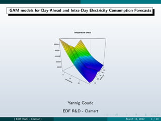
  • 1. GAM models for Day-Ahead and Intra-Day Electricity Consumption Forecasts Temperature Effect 65000 60000 55000 z 50000 45000 50 40 0 30 d .in ek we 10 20 we ek.t em p 20 10 Yannig Goude EDF R&D - Clamart ( EDF R&D - Clamart) March 15, 2012 1 / 24
  • 2. Motivation of Electricity Load Forecasting Electricity can not be stored, thus forecast- ing elec. consumption: to avoid blackouts on the grid to avoid financial penalties to optimize the management of production units and electricity trading Managing a wild variety of production units: nuclear plants fuel, coal and gas plants renewable energy: water dams, wind farms, solar panels... ( EDF R&D - Clamart) March 15, 2012 2 / 24
  • 3. Motivation of Electricity Load Forecasting Short-term load forecasting: from 1 day to a few hours horizon ( EDF R&D - Clamart) March 15, 2012 3 / 24
  • 4. (Generalized) Additive smooth models consider a univariate response y and corresponding predictors x1 , ..., xp an additive smooth model has the following structure: yi = Xi β + f1 (x1,i ) + f2 (x2,i ) + f3 (x3,i , x4,i ) + ... + εi Xi β is the linear part of the model functions fj are supposed to be smooth εi : iid E (εi ) = 0,V (εi ) = σ 2 normality if needed (tests...) More precisely, we want to solve the following pb: minβ,fj ||y − X β − f1 (x1 ) − f2 (x2 ) + ...)2 + λ1 f1 (x)2 dx + λ2 f2 (x)2 dx + ... ( EDF R&D - Clamart) March 15, 2012 4 / 24
  • 5. (Generalized) Additive smooth models Estimation of the fj : basis expansion in a spline basis kj fj (x) = aj,q (x)βj,q q=1 Then the additive model becomes k1 k2 yi = Xi β + a1,q (x)β1,q + a2,q (x)β2,q + ... + εi q=1 q=1 Unknowns: choice of the spline basis, number-position of knots kj β and aj,q ⇒ take large kj and proceed to penalized regression (ridge) ( EDF R&D - Clamart) March 15, 2012 5 / 24
  • 6. (Generalized) Additive smooth models Then the initial problem minβ,fj ||y − X β − f1 (x1 ) − f2 (x2 ) + ...)2 + λ1 f1 (x)2 dx + λ2 f2 (x)2 dx + ... becomes a linear regression problem: minβ ||y − X β||2 + λ j β T Sj β as fj (x)2 dx can be written as β T Sj β absorbing aj,q (xi ) into Xi Solution: βλ = (X T X + λj Sj )−1 X T y ( EDF R&D - Clamart) March 15, 2012 6 / 24
  • 7. (Generalized) Additive smooth models How to choose the penalization parameter λ? without any penalisation: β0 = (X T X )−1 X T y regularised: βλ = (X T X + λj Sj )−1 X T y β λ = Fλ β 0 Where Fλ = (X T X + λj Sj )−1 X T X tr (Fλ ): estimated degrees of freedom ( EDF R&D - Clamart) March 15, 2012 7 / 24
  • 8. (Generalized) Additive smooth models How to choose the penalization parameter λ? ( EDF R&D - Clamart) March 15, 2012 8 / 24
  • 9. (Generalized) Additive smooth models Ordinary Cross Validation leave one observation yi estimate a model µ−i on the new data set forecast yi with µ−i i do that for all i choose the λ that minimizes the OCV score: n V0 (λ) = (yi − µ−i )2 /n i i=1 Pb: calculation time Generalized Cross Validation [Craven and Wahba (1979)] Vg (λ) = n y − X βλ |2 /(n − tr (Fλ ))2 Advantages of GCV: λ is obtained by numerical minimization of Vg (few comp. cost) Vg (λ) is invariant when doing useful transf. of the data (on-line update, big data) ⇒ Software: R, package mgcv (see[Wood (2001)] and [Wood (2006)]) ( EDF R&D - Clamart) March 15, 2012 9 / 24
  • 10. From GAM to BAM BAM: Big Additive Models ⇒ for huge data sets (more than 10 000 observations) we use the QR decomposition: X = QR, f = Q T y and denote ||r ||2 = ||y ||2 − ||f ||2 Q orth. matrix, R upper triang. then we have: n||f − R βλ ||2 + ||r ||2 Vg (λ) = (n − tr (Fλ ))2 where Fλ is now (R T R + λj Sj )−1 R T R ⇒ Once we have R, f and ||r ||2 , X plays no further part ( EDF R&D - Clamart) March 15, 2012 10 / 24
  • 11. From GAM to BAM ⇒ Application for large data sets: X0 y0 X is too big and has to be split: , similarly y = X1 y1 R0 form QR dec. X 0 = Q0 X0 and = Q1 R see section 12.5 of X1 [Golub and Van Loan (1996)] T Q0 0 Q0 y0 then X = QR with Q = Q1 and Q T y = Q1 T 0 I y1 ⇒ On-line update X0 , y0 past data, X1 , y1 last observations Use the new data X1 , y1 to update R, f and ||r ||2 Re-estimate λ and βλ (previous values can be used as starting values for the numerical optimization) ( EDF R&D - Clamart) March 15, 2012 11 / 24
  • 12. ( EDF R&D - Clamart) 40000 50000 60000 70000 80000 90000 1/9/2002 13/1/2003 28/5/2003 9/10/2003 21/2/2004 4/7/2004 16/11/2004 31/3/2005 Application to Electricity Load Data 12/8/2005 25/12/2005 Trend 8/5/2006 20/9/2006 1/2/2007 16/6/2007 28/10/2007 Electricity Data 10/3/2008 23/7/2008 4/12/2008 18/4/2009 31/8/2009 March 15, 2012 12 / 24
  • 13. ( EDF R&D - Clamart) 30000 40000 50000 60000 70000 80000 1/1/2006 20/1/2006 8/2/2006 27/2/2006 18/3/2006 7/4/2006 26/4/2006 15/5/2006 Application to Electricity Load Data 3/6/2006 22/6/2006 12/7/2006 31/7/2006 19/8/2006 Yearly Pattern 7/9/2006 26/9/2006 Electricity Data 16/10/2006 4/11/2006 23/11/2006 12/12/2006 31/12/2006 March 15, 2012 13 / 24
  • 14. ( EDF R&D - Clamart) 35000 40000 45000 50000 55000 1/6/2006 2/6/2006 4/6/2006 5/6/2006 7/6/2006 8/6/2006 10/6/2006 12/6/2006 Application to Electricity Load Data 13/6/2006 15/6/2006 16/6/2006 18/6/2006 19/6/2006 Weekly Pattern 21/6/2006 23/6/2006 Electricity Data 24/6/2006 26/6/2006 27/6/2006 29/6/2006 30/6/2006 March 15, 2012 14 / 24
  • 15. Application to Electricity Load Data Electricity Data Daily Pattern 70000 Mo Fr Tu Sa 65000 We Su 60000 55000 Th Load 50000 45000 40000 0 10 20 30 40 Instant ( EDF R&D - Clamart) March 15, 2012 15 / 24
  • 16. Load (MW) 60000 65000 70000 75000 80000 0 10 Normal ( EDF R&D - Clamart) 20 Instant 30 Special Tariff 40 Application to Electricity Load Data 55000 60000 65000 70000 75000 80000 85000 Special Days 20/12/2007 20/12/2007 21/12/2007 Electricity Data 22/12/2007 23/12/2007 24/12/2007 25/12/2007 25/12/2007 26/12/2007 27/12/2007 28/12/2007 29/12/2007 30/12/2007 30/12/2007 31/12/2007 1/1/2008 2/1/2008 3/1/2008 4/1/2008 4/1/2008 March 15, 2012 16 / 24
  • 17. Application to Electricity Load Data Electricity Data Load-Temperature ( EDF R&D - Clamart) March 15, 2012 17 / 24
  • 18. Application to Electricity Load Data Electricity Data 75000 Load-Cloud Cover 8 70000 6 Cloud cover (Octets) Load (MW) 65000 4 2 60000 0 0 10 20 30 40 0 10 20 30 40 Instant Instant ( EDF R&D - Clamart) March 15, 2012 18 / 24
  • 19. Application to Electricity Load Data Model Lt = f1 (Lt−48 , It ) IHH +f2 (Lt−48 , It ) IHW +f3 (Lt−48 , It ) IWH +f4 (Lt−48 , It ) IWW + g1 (Tt , It ) + g2 (Tt−48 , Tt−96 ) + g3 (Cloudt ) + h(Toyt , It ) 48 + i=1 γi Spec.Tarift 11 + j=1 αj + s(t) + εt fj s: lagged load effects gj s: meteo. effects hs: yearly pattern, Toy is time of year γi : special tariff effect by half-hour of the day αj mean load for: sunday, monday, tuesday,...,saturday, HH,HW,WH and WW days s(t) is the trend Estimation period: september 2002 - august 2008 Forecasting period: september 2008 - august 2009 ( EDF R&D - Clamart) March 15, 2012 19 / 24
  • 20. Application to Electricity Load Data Model GAM Model 10000 Temperature Effect 5000 70000 65000 Load (MW) 0 L[t] 60000 −5000 55000 50000 40 30 30 −10000 20 20 I[t] T[t 10 Mo Fr Su ] 10 0 we Sa 0 0 10 20 30 40 Hour Yearly Cycle Trend 10000 80000 70000 5000 60000 z 0 50000 40000 −5000 40 0.0 30 0.2 0.4 20 nt Po sta san 0.6 In 10 −10000 0.8 0 120000 140000 160000 180000 200000 220000 240000 t ( EDF R&D - Clamart) March 15, 2012 20 / 24
  • 21. Application to Electricity Load Data Model Lagged Load Effect, WW Lagged Load Effect, WH 80000 70000 70000 60000 L[t] 60000 L[t] 50000 50000 40000 40000 40 30000 40 80000 30 80000 30 70000 20 70000 20 60000 60000 ] ] I[t I[t L[t 50000 10 L[t 50000 10 −1 −1 ] 40000 ] 40000 30000 0 30000 0 Lagged Load Effect, HW Lagged Load Effect, HH 30000 20000 80000 L[t] 10000 L[t] 60000 0 −10000 40000 40 40 80000 30 80000 30 70000 20 70000 20 60000 60000 ] ] I[t I[t L[t 50000 10 L[t 50000 10 −1 −1 ] 40000 ] 40000 30000 0 30000 0 ( EDF R&D - Clamart) March 15, 2012 21 / 24
  • 22. RMSE (MW) −8000 −4000 0 2000 4000 6000 500 1000 1500 2000 0 9/1/2002 Figure: 12/19/2002 4/8/2003 ( EDF R&D - Clamart) 8/12/2003 10 12/4/2003 3/22/2004 7/26/2004 11/17/2004 20 3/7/2005 7/6/2005 Tu Th Mo We 10/23/2005 Instant 2/18/2006 30 6/20/2006 Fr 10/8/2006 Su Sa 2/3/2007 6/4/2007 40 9/21/2007 1/17/2008 5/6/2008 8/31/2008 Application to Electricity Load Data MAPE (%) −8000 −4000 0 2000 4000 6000 0.5 1.0 1.5 2.0 2.5 3.0 Model 0 0 10 10 20 20 Instant 30 30 Tu Th Mo We 40 40 Fr Su Sa Top: half hourly RMSE (left) and MAPE (right) by type of day. Bottom: residuals March 15, 2012 22 / 24
  • 23. Application to Electricity Load Data Model Performances Model RMSE (MW) MAPE (%) RGCV score Estimation set m0 831 1.17 882 m1 1024 1.46 806 Forecasting set m0 1220 1.87 On-line m0 1048 1.49 m1 1156 1.62 On-line m1 1109 1.53 ( EDF R&D - Clamart) March 15, 2012 23 / 24
  • 24. Application to Electricity Load Data Model Residuals 0 −100 −200 −300 m0 m1 On−line update −400 −500 −600 9/1/2008 9/17/2008 10/4/2008 10/21/2008 11/15/2008 12/2/2008 12/19/2008 1/13/2009 1/30/2009 2/16/2009 3/4/2009 3/21/2009 4/7/2009 4/28/2009 5/27/2009 6/17/2009 7/4/2009 7/25/2009 8/11/2009 8/31/2009 Figure: Cumulative residuals (right) for models m0 (black), m1 (red), and their on-line updated version (dashed lines). ( EDF R&D - Clamart) March 15, 2012 24 / 24
  • 25. Application to Electricity Load Data Model Craven and Wahba (1979) ”Smoothing noisy data with spline functions: estimated the correct degree of smoothing by the method of general cross validation”. Numerische Mathematik 31, 377-403. Golub and Van Loan (1996) ”Matrix Computations, 3rd edition”. John Hopkins Studies in the Mathematical Sciences. Green and Silverman (1994) ”Nonparametric Regression and Generalized Linear Models”. Chapman and Hall. Hastie and Tibshirani (1990) ” Generalized Additive Models”. Chapman and Hall. Pierrot and Goude (2011) ”Short-Term Electricity Load Forecasting With Generalized Additive Models”, Proceedings of ISAP power 2011. Wahba (1990) ”Spline Models of Observational Data”. SIAM Wood (2001) mgcv:GAMs and Generalized Ridge Regression for R. R News 1(2):20-25 Wood and Augustin (2002) ”GAMs with integrated model selection using penalized regression splines and applications to environmental modelling”. Ecological Modelling 157:157-177 Wood (2006)Generalized Additive Models, An Introduction with R (Chapman and Hall, 2006) ( EDF R&D - Clamart) March 15, 2012 24 / 24