1. Journal of Marine Systems 74 (2008) 585–591
Contents lists available at ScienceDirect
Journal of Marine Systems
j o u r n a l h o m e p a g e : w w w. e l s ev i e r. c o m / l o c a t e / j m a r s y s
On the influence of large wind farms on the upper ocean circulation
Göran Broström
Norwegian Meteorological Institute, Postboks 43 Blindern, N-0313 OSLO, Norway
a r t i c l e i n f o a b s t r a c t
Article history: Large wind farms exert a significant disturbance on the wind speed in the vicinity of the
Received 21 May 2007 installation and in this study we outline the oceanic response to the wind wake from a large
Received in revised form 25 April 2008 wind farm placed in the ocean. We find that the size of the wind wake is an important factor for
Accepted 2 May 2008
the oceanic response to the wind farm. We show through simple analytical models and
Available online 15 May 2008
idealized numerical experiments that a wind speed of 5–10 m/s may generate upwelling/
downwelling velocities exceeding 1 m/day if the characteristic width of the wind wake is of the
Keywords:
Wind farm
same size or larger than the internal radius of deformation. The generated upwelling is
Wind forcing sufficiently enough that the local ecosystem will most likely be strongly influenced by the
Upwelling presence of a wind farm.
Ocean dynamics © 2008 Elsevier B.V. All rights reserved.
1. Introduction Knudsen et al., 1992; Karlsen et al., 2004; Hastings and
Popper, 2005), shadowing from the wind mills, and bird and
It is predicted that large open-water wind farms will bat collisions with the wind mills (Tucker, 1996a,b; Garthe
become much more frequent in the decades to come (Archer and Hüppop, 2004; Wiggelinkhuizen et al., 2006). There is
and Jacobson, 2003, 2005; Henderson et al., 2003; Kooijman probably also an influence of the wind farm on the local
et al., 2003; Hasager et al., 2006). There are certain advantages climate (Baidya Roy and Pacala, 2004; Rooijmans, 2004) as
with oceanic wind farms, not least the higher wind speeds well as on the global climate if wind farms become abundant
and locations away from densely populated areas. On the (Keith et al., 2004).
negative side are large costs of establishing and maintaining In this study we outline how the presence of a large wind
wind farms out in the open water (Byrne and Houlsby, 2003), farm, which changes the wind stress at the sea surface, affects
wave forces on the structures, disturbance of ship traffic, and the upper ocean response to wind forcing. Using general
environmental effects among others. theoretical arguments we show that large wind farms may
Although there are a number of plans and studies for large have a direct, and strong, impact on the circulation pattern
wind farms in the open ocean the environmental conse- around the installation. In particular, if the wind farm is large
quence are not well known and much of the literature is in a enough variations in the wind will create upwelling and
so called gray form represented by reports, theses etc. downwelling patterns around the wind farm through diver-
Presently, the environmental focus has mainly been on the gence in the Ekman transport. The main theoretical descrip-
direct consequences of the solid structures of the wind farm tion is based on the so called reduced gravity model, which
on the oceanic environment. The establishment of solid describes the dynamics of a buoyant layer on top of a dense
structures will probably act as artificial reefs creating new stagnant layer. The theoretical framework follows standard
highly productive areas in the sea. Other possible environ- derivations used in the geophysical fluid dynamics (Gill, 1982;
mental consequences may be the impact of electric cables on Pedlosky, 1987) and the analysis shows that the oceanic
the fish migrations (Branover et al., 1971; Wiltschko and response is more sensitive to the curl of the wind stress than
Wiltschko, 1995), effects of sound generated by the power to the wind stress itself. In the open ocean, the curl of the
plant on the fauna (Sand and Karlsen, 1986; Karlsen, 1992; wind stress is usually relatively small as the gradients in the
wind forcing are set by the scale of atmospheric low-pressure
systems, which are much larger than the corresponding
E-mail address: goran.brostrom@met.no. dynamical scales of the ocean. The presence of a wind farm
0924-7963/$ – see front matter © 2008 Elsevier B.V. All rights reserved.
doi:10.1016/j.jmarsys.2008.05.001

2. 586 G. Broström / Journal of Marine Systems 74 (2008) 585–591
will generate an unnaturally strong horizontal shear in the farm creates a disturbance that is strongest in the y-direction.
wind stress, which creates a large curl of the wind stress that We will consider two simple forms of the wind stress: 1) A
causes a divergence/convergence in the upper ocean. We find wind stress that is homogenous in the x-direction such that
that the impact on the ocean currents will increase with the analytical solutions can be found and 2) a wind wind-stress
size of the wind farm, and when the size is comparable with pattern having a more realistic two-dimensional form. The
the internal radius of deformation (or internal Rossby radius) stresses are given by
we expect to find a circulation, and an associated upwelling
2
pattern, to be excited by the wind farm. Using a simple τ x ¼ τx0 −Δτ x e−ð 2y=LÞ ;
2 À Á ð1a; bÞ
example we show that a wind speed of 5–10 m/s can induce τ x ¼ τx0 −Δτ x e−ð 2y=ð0:8Lþ0:2xÞÞ max e−ð1−xÞ=L x=L; 0 ;
an upwelling exceeding 1/m day. It is well known that
upwelling can have significant impact on the local ecosystem where τx0 is the wind stress outside the influence of the wind
(e.g., Okkonen and Niebauer, 1995; Valiela, 1995; Botsford farm, Δτx reflect the change in the wind stress induced by the
et al., 2003; Dugdale et al., 2006). Thus, as upwelling of wind farm, and L is the characteristic size of the wind farm.
nutrient rich deep water represent the main source of For the more realistic scenario we assume that the wind
nutrients during summer in most oceanic areas it is likely deficit is zero at the upwind end of the wind farm, reaches a
that the upwelling induced by a wind farm will imply an maximum at the end of the farm and declines downwind
increased primary production, which may affect the local from the farm with a characteristic length scale L. We also
ecosystem. assume that the width of the wind deficit increases in the
There are some notable similarities between the proposed downwind direction, as expected from turbulent mixing and
upwelling process and some natural upwelling systems meandering of the wake. The shapes of the proposed wind
generated by divergence in the Ekman transport due to stresses are shown in Fig. (1), and follow loosely results from
wind curls at coastal boundaries (Dugdale et al., 2006; Fennel recent studies (Barthelmie et al., 2003; Corten and Brand,
and Lass 2007) or the marginal ice zone (MIZ) (Røed and 2004; Corten et al., 2004; Hegberg et al., 2004; Christiansen
O'Brian, 1983; Okkonen and Niebauer, 1995; Fennel and and Hasager, 2005; Hasager et al., 2006). However, it should
Johannessen, 1998). For the present scenario, the MIZ studies
are probably most relevant: Røed and O'Brian (1983)
estimated upwelling velocities of order 5 m/day for reason-
able wind speeds while Okkonen and Niebauer (1995)
invoked upwelling velocities of up to 8 m/day, which were
seen to fuel an extensive bloom in the MIZ.
In Section 2, the basic equations that describe the
structure of the oceanic response to wind forcing in the
vicinity of a wind farm are outlined. Some dynamical features
of these equations are described in Section 3, while Section 4
is devoted to discussion of the results.
2. Basic equations
In this section we will outline some simple equations that
describe a buoyant surface layer on top of a stagnant deep
layer; these equations are very similar to the equations
describing the barotropic flow and are generally referred to as
the reduced gravity model, or a 1 1/2 layer model. The model
is based on integration over the active upper layer and is thus
two-dimensional; vertical velocity is manifested as a vertical
movement of the pycnocline and is thus included implicitly. It
should be remembered that certain conditions must be
fulfilled for the reduced gravity model to be valid; the
reasonableness of these assumptions can be questioned for
the outlined scenarios. However, the reduced gravity model
highlights a number of processes that may be important in
the vicinity of large wind farms, and the primary aim of the
present study is to outline the basic response of the upper
ocean to a large wind farm, not to describe these processes in
detail.
2.1. Form and strength of wind drag
Fig. 1. The wind-stress deficit used in this study. a) Cross section of the one
The form and strength of the perturbations in the wind one-dimensional case used for analytical studies and b) map of the more
stress is the basic driving mechanism of this study. The wind realistic wind-stress deficit, where also the extent of the wind farm is
stresses used in this study are in the x-direction and the wind displayed by a black line.

3. G. Broström / Journal of Marine Systems 74 (2008) 585–591 587
be noted that further investigations focusing on the wind relatively shallow water. As a final remark it may seem strange
stress at the sea surface are required for more accurate that the gradient of the slope at the lower boundary appears to
predictions, and specifications, of how a large wind farm induce a force in the upper layer; the force comes really from
influence the wind stress at the sea surface. the sloping surface and the slope in the lower layer only
removes the pressure gradient from the surface down into the
2.2. Basic shallow water equations stagnant deep layer. However, the changes in the surface
elevation are small and can be neglected in the remaining
Let us consider an ocean that rotates with the angular analysis, and this is the rigid lid approximation.
speed f/2, where f is the Coriolis parameter, and having an
active upper layer with thickness h and density ρ − Δρ 2.3. General equation for h
overlying an infinitely deep passive layer with density ρ.
The horizontal coordinates are x and y; the vertical coordinate The response of the thickness of the upper layer to wind
is z, which is zero at the sea surface and positive upwards. The forcing is the key feature in the reduced gravity model. If the
bottom of the active layer is located at z = −h(x,y) while the thickness of the upper layer is known, the velocities of the
free surface is located at z = 0 according to the rigid lid system are easily calculated. After some manipulations of
approximation (see Fig. 2). Eq. (2) we find (Gill, 1982; Pedlosky, 1987)
The flow in the active upper layer can be described by " ! #
integrating the Navier-Stokes and continuity equations from ∂ ∂2 2 f 1∂
þ f h−r Á ð gh0 rhÞ ¼ − curlðτ Þ− r Á τ: ð3Þ
the bottom of the active layer to the surface, and by applying ∂t ∂t 2 ρ ρ ∂t
the hydrostatic approximation. Neglecting the non-linear
terms for simplicity (although it should be recognized that Eq. (3) is very general and describes an extensive set of
they are in general not negligible), the linear reduced gravity phenomena where the reduced gravity approximation is
equations in transport form become valid. A normal problem in using this equation is to find
appropriate boundary conditions (Gill, 1982; Pedlosky, 1987);
∂U ∂h 1 for the reduced gravity model we will simply assume that
−fV ¼ −g 0 h0 þ τ x ;
∂t ∂x ρ h = h0 at the boundaries or that it is bounded at infinity.
∂V 0 ∂h 1 In the following analysis we will neglect fast transients such
þ fU ¼ −g h0 þ τy ; ð2a–cÞ
∂t ∂y ρ that the second order time derivative in Eq. (3) can be neglected
∂h ∂U ∂V
þ þ ¼ 0; (i.e., we neglect internal gravity waves, the geostrophic
∂t ∂x ∂y
adjustment process and all processes for small time t b f).
where U and V are the mass transports in x and y directions, Furthermore we assume that the wind forcing is constant and
respectively, g' =gΔρ/ρ is the reduced gravity, h0 is the initial neglect the last term. It is convenient to use non-dimensional
thickness of the upper layer and we will assume that h0 = const, variables and we thus introduce the scales t =t'f− 1, (x,y) = (x',y')L,
S B S B
τx, τy = (τx −τx ,τy −τy ) are the stresses acting on the water and h =h'Δτ/fρL: We have (dropping the primes on the non-
S S B B
column where τx , τy , are the surface stresses and τx , τy are the dimensional variables)
B B
stresses at the bottom of the active layer (τx , τy are assumed to τ
be zero in this study). An important assumption for the reduced ∂À Á
h−a2 r2 h ¼ −curl ; ð4Þ
gravity model is that the bottom layer should be deep and ∂t Δτ
pffiffiffiffiffiffiffiffiffiffi
stagnant; furthermore, the amplitude in h must be small: These where a ¼ g 0 h0 =fL is a non-dimensional number (here
assumptions may be questionable for wind farms placed in considered as constant) identified as the internal radius of
deformation, or the internal Rossby radius, divided by the
size of the wind farm. Eq. (4) is easily integrated in time
such that
τ
ðh−h0 Þ−a2 r2 ðh−h0 Þ ¼ −tcurl ; ð5Þ
Δτ
where h0 is the initial non-dimensional depth of the
pycnocline. For the one-dimensional case there exists an
analytical solution whereas we solve this equation numeri-
cally for two dimensions. The important lesson to be learnt
from Eq. (5) is that the depth of the pycnocline changes
linearly in time, i.e., (h − h0)/t has a self-similar solution, and
that the rate depends linearly on the strength of the wind-
stress curl.
3. Some dynamical features of the equations
3.1. Analytical time-dependent solution for zonal wind forcing
In this section we aim at finding some analytical results. To
Fig. 2. Schematic picture of the geometric settings used in this study. highlight the ocean response to wind forcing we consider a

4. 588 G. Broström / Journal of Marine Systems 74 (2008) 585–591
wind distribution in the form of a Gaussian, as outlined by
Eq. (1a). From Eq. (5) we find that
∂2 1 ∂τx
ðh−h0 Þ−a2 ðh−h0 Þ ¼ −t : ð6Þ
∂y2 Δτ x ∂y
To obtain the full structure of the solution it is necessary to
also solve an inhomogeneous Helmholtz equation. Assuming
that the wind stress has a Gaussian distribution (Eq. (1a)), and
by requiring that the solution is bounded at infinity we find
the following solution
pffiffiffi
½
π − 12 2y 1
hðt; yÞ−h0 ¼t e 8a e a 1− erfc þ 2y
16a2 4a
ð7Þ
2y
−e− a 1− erfc
1
4a
þ 2y Š
Fig. 4. The spatial structure of the disturbance in thickness of the upper layer
where erfc is the error function. The disturbance of the upper for a2 = 1 and t = 1. Gray lines represent the wake in the wind forcing.
layer thickness thus increases linearly with time and is
proportional to the magnitude of the wake. Due to the
dynamics of the geostrophic adjustment process the signal deformation radius is compared to the size of the wind farm).
has a form that depends on the non-dimensional parameter a If the variation in wind has a length scale that is much larger
(Fig. 3) (again a is a measure of how large the internal than the internal deformation radius the form of the
disturbance is fully governed by the form of the wind curl
(as seen by setting a = 0 in Eq. (6)). However, if the structure of
the wind field is of the same, or smaller, dimension than the
internal deformation radius the ocean responds by distribut-
ing the signal over an area with a characteristic width
corresponding to the internal deformation radius. It should
also be noted that the amplitude of the signal becomes
smaller for large values of a2.
3.2. More general time-dependent numerical solution
In two dimensions it is more difficult to find analytical
solutions and we rely on numerical solutions using the self
adapting finite element technique implemented in FEMLAB®
package, the relative tolerance was set to 10− 6 and two
refinements of the grid were made (the self adaptation
implies that the resolution will depend on the parameter a2).
It should be remembered that the linear solution predicts that
the shape of the response is self-similar and will not change in
Fig. 3. a) The form of the disturbance in thickness of the upper layer and b)
the geostrophic velocity for various number of the a2 parameter (here the Fig. 5. Section of the disturbance in thickness of the upper layer at the
wind forcing is given by τx = e− (2y) ).
2
downwind end of the wind farm.

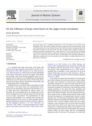
5. G. Broström / Journal of Marine Systems 74 (2008) 585–591 589
for a2 = 1 the amplitude is about 25% of the amplitude for
small a2. Apparently, the geostrophic adjustment process
mixes the positive and negative response appearing on each
side of the wind wake such that the magnitude of the
response becomes weaker. It is a notable feature that the
response for increasing value of a2 becomes wider as well. A
key parameter for the environmental influence is the strength
of the upwelling and the maximum value of the pycnocline
height as a function of a2 is shown in Fig. (6). Again we see
that the amplitude of the response decreases rapidly with a2,
showing that a key parameter for the ocean response is the
physical size of the wind wake.
Inserting f = 1.2 · 10− 4 s− 1, h0 = 10 m, Δρ = 2 kg/m3, we find
that the internal radius of deformation is 3.7 km and using
Fig. 6. The maximum amplitude of the disturbance in thickness of the upper L = 5 km we find a2 ≈ 0.54, which implies that there should be
layer as a function of a2. an important signal from a 5 km wide wind farm on the
upwelling pattern. The upwelling velocity can be estimated
time and we evaluate the solution at t = 1 (Fig. 4). From Fig. (5) from the horizontal shear in the wind wind-stress times the
we see that the pycnocline will rise on the southern side of spatial distribution/influence of the response as outlined in
the wind farm and will be depressed on the northern side. The Figs. (5) and (6), and we thus expect the maximum upwelling
ocean response follows the wind pattern to a large degree, velocity to be roughly Δτx/(ρfL)·0.3 ≈ 1 m/day for the case with
although the signal covers a slightly larger area than the wind Δτx = 0.025 N/m2, and a2 ≈ 0.54. It should be noted that this
wake as expected from the geostrophic adjustment process. only gives a very rough estimate of the upwelling velocity.
The spatial response depends critically on the deformation When the disturbances grow larger it is expected that non-
radius, and cross sections of the pycnocline position at x = 1 (at linear terms, lower-layer motions, and bottom friction
the downwind end of the wind farm) are displayed in Fig. (5); become important. Anyway, the predicted upwelling velocity
Fig. 7. The spatial structure of the disturbance in the mixed layer depth after 1 day (left panels) and 5 days (right panels) for wind forcing τx0 = 0.05 N/m2,
Δτx = 0.025 N/m2 (upper panels), and τx0 = 0.1 N/m2, Δτx = 0.05 N/m2, (lower panels).

6. 590 G. Broström / Journal of Marine Systems 74 (2008) 585–591
would provide a very strong forcing on the ecosystem in the possible explanation is that the upwelling leads to a cyclonic
vicinity of the wind farm during typical summer situations. circulation while the downwelling generates an anti-cyclonic
circulation. It is known in geophysical fluid dynamics that
3.3. Results from a general circulation model there are certain differences between cyclonic and anti-
cyclonic eddies. However, an analysis of the dipole structure
We end this section by showing results from some simple seen in these experiments is beyond the scope of the present
experiments carried out with the MITgcm general circulation study.
model (Marshall et al., 1997a,b), which provides a non-linear as
well as a full three-dimensional solution; we use the model in 4. Results and discussion
its hydrostatic mode although it has non-hydrostatic capability.
To describe mixing in the upper ocean we apply the KPP The demand for electric power has stimulated many plans
turbulence mixing scheme (Large et al., 1994). We here assume for constructing large off-shore wind-power plants. However,
that L = 5 km and that the ocean is 20 m deep, and we apply no there have only been a few studies on the environmental
slip condition at the bottom (notably the KPP model will impact of these wind farms on the oceanic environment; most
calculate the velocity at the first grid point according to a available studies describe the direct effects of the wind mill
quadratic law). The temperature is 10 °C below −10 m and is constructions, noise and shadowing from the installations,
20 °C above −10 m, and we use a linear equation of state such and the possible influence of electric cables on the marine life.
that ρ =ρ0(1 −αT), where ρ0 = 1000 kg m− 3 and α = 2 · 10− 4 K− 1. In this study we outline a possible environmental influence of
f = 1.2 · 10− 4 is taken as constant. The horizontal resolution is the wind farms that, to our knowledge, has not previously
200 m and the domain stretches from x = −5L to 15L and from been described in any detail in the scientific literature. More
y = −10L to 10L, and we apply periodic boundary conditions. In specifically, the wind farms may influence the wind pattern
the vertical we use 0.5 m resolution. The wind is applied and hence force an upper ocean divergence. This will in turn
instantaneously to an ocean at rest. influence the upwelling pattern, thereby changing, for
To visualize the ocean response to the wind forcing we instance, the temperature structure and availability of
define the following quantity nutrients in the vicinity of the wind farm.
The basic oceanic response depends on the reduction in
1
ΔHml ¼ h0 − ∫ 0 ðT−TB Þdz; ð8Þ the wind stress at the sea surface, both in magnitude and the
TU −TB −H
size of the affected area. From a literature review it appears
where h0 = 10 m is the initial position of the thermocline, (TU, that these quantities have not yet been studied in sufficiently
TB) = (20,10) °C is the initial temperature of the upper and detail to provide a reliable description of these features. Most
lower layers, respectively. The right-hand side of Eq. (6) will studies of wind-farm influence on the wind focuses on the
essentially measure the depth of the 10 °C isotherm, and wind structure within the farm and how it will affect the
subtracting this from the initial position of the 10 °C isotherm efficiency of the wind farm. However, the far-reaching wind
ΔHml will measure the amount of upwelling at a certain deficit and the wind stress at the sea surface have not been
location. subjected to in substantial investigations. Thus, it is probably
The distributions of ΔHml after 1 resp. 5 days and a wind necessary with complementing studies of these issues before
stress corresponding roughly to a wind speed 5 and 7.5 m/s accurate estimates of the influence on the upper ocean
(using a drag coefficient of 1.5 · 10− 3) are displayed in Fig. (7). physics can be established. Here, it should also be underlined
The initial magnitude of the upwelling/downwelling is on the that the size of the wind farm is a very important factor and
order of 0.8 m/day for the weak wind case, and is about 1.5 m/ that the oceanic response rapidly becomes much stronger
day for the strong wind case (Fig. 7a, c) in rough agreement when the size of the wind farm becomes larger than the
with the theoretical estimates presented in Section 3.2 (i.e., internal radius of deformation.
1 m/day and 2 m/day, respectively). However, after some time, Examples of how divergence of the wind causes upwelling
say 2–3 days, the response becomes weaker, this weakening in the ocean are when winds blow along a coast, over an
being most evident in the strong wind-forcing case. Most island, or along the MIZ (Gill, 1982; Røed and O'Brian, 1983;
likely, non-linear effects become important as the amplitude Okkonen and Niebauer, 1995; Valiela, 1995; Botsford et al.,
of the disturbance grows. (The Rossby number (U/Lf) that 2003; Dugdale et al., 2006). With a wind-driven transport
measures the importance of non-linear terms relative to the directed out from the coast the water that is transported out
Coriolis force is of order unity for U = 0.6 m/s, furthermore the from the coast will be replaced by water from deeper layers
movements of the pycnocline are not negligible; we thus through upwelling. These types of systems and the ecosystem
expect that the non-linear terms are important, but they do response to the upwelling of nutrient rich, but also plankton
not dominate the system). Internal friction may be important poor, deep water have been studied extensively (Valiela, 1995;
but due to weak velocities in the lower layer we do not expect Botsford et al., 2003; Dugdale et al., 2006). However, there is
bottom friction to be important. Furthermore, it is clear from an important difference between the upwelling forced along a
the numerical experiments that the shape of the disturbance coast and the type of upwelling that may be forced by large
changes and become wider with time. wind farms. In the coastal upwelling case, the presence of
Another striking property of the numerical model solution land implies that the ecosystem properties cannot be
is that the response tends to become asymmetric with time, supplied from upstream condition; the wind-farm induced
which is not predicted by the linear model. Notably, the upwelling on the other hand, has an important upstream
depression of the pycnocline is wider and by smaller import of water that carries the properties of the ecosystem.
amplitude than the response in the upwelling sector. A The situation along the MIZ is probably more relevant but has

7. G. Broström / Journal of Marine Systems 74 (2008) 585–591 591
not been studied to the same degree; one difference here is Corten, G.P., Schaak, P., Hegberg, T., 2004. Velocity Profiles Measured Above a
Scaled Windfarm. Energy Research Centre of the Netherlands. ECN-RX-
that the position of MIZ change with time and reacts to the 04-123.
wind forcing while a wind farm has a fixed position. Dewar, W.K., 1998. Topography and barotropic transport control by bottom
We have not outlined the barotropic response in this friction. J. Mar. Res. 56, 295–328.
Dugdale, R.C., Wilkerson, F.P., Hogue, V.E., Marchi, A., 2006. Nutrient controls
study; this response is somewhat different but needs to be on new production in the Bodega Bay, California, coastal upwelling
addressed. To the lowest order approximation the geostrophic plume. Deep-Sea Res. 53, 3049–3062.
balance inhabits vertical movements and the flow follows Fennel, W., Johannessen, O.M., 1998. Wind forced oceanic responses near ice
edges revisited. J. Mar. Syst. 14, 57–79.
depth contours, or more specifically closed f/H contours. The
Fennel, W., Lass, H.U., 2007. On the impact of wind curls on coastal currents.
basic steady state balance is characterized by a state where J. Mar. Syst. 68, 128–142.
the net divergence over a closed f/H contour due to wind Garthe, S., Hüppop, O., 2004. Scaling possible adverse effect of marine wind
farms on seabirds: developing and applying a vulnerability index. J. Appl.
forcing is balanced by the net divergence induced by the
Ecol. 41, 724–734.
Ekman layer at the bottom (Walin, 1972; Dewar, 1998; Nøst Gill, A.E., 1982. Atmosphere–Ocean Dynamics. Academic Press, Inc., London.
and Isachsen, 2003). It should be noted that the divergence of 662 pp.
the wind field is generally small given the large size of Hasager, C.B., Barthelmie, R.J., Christiansen, M.B., Nielsen, M., Pryor, S.C.,
2006. Quantifying offshore wind resources from satellite wind maps:
atmospheric low-pressure systems. Accordingly, the wind study area the North Sea. Wind Energy 9, 63–74.
tends to generate relatively weak barotropic signals around Hastings, M.C., Popper, A.N., 2005. Effects of Sound on Fish. http://www.dot.
depth contours having small horizontal scales (say 100 km). ca.gov/hq/env/bio/files/Effects_of_Sound_on_Fish23Aug05.pdf. Contract
43A0139 Task Order, 1, California Department of Transportation.
The presence of a wind farm may create a substantial Hegberg, T., Corten, G.P., Eecen, P.J., 2004. Turbine Interaction in Large
divergence of the wind field in the immediate vicinity of the Offshore Wind Farms; Wind Tunnel Measurements. ECN-C-04-048,
wind farm. If the farm is placed close to a sloping bottom it is Energy Research Centre of the Netherlands.
Henderson, A.R., et al., 2003. Offshore wind energy in Europe — a review of
thus possible that the wind farm may provide a substantial the state-of-the-art. Wind Energy 6, 35–52. doi:10.1002/we.82.
additional forcing of the barotropic-current system in an Karlsen, H.E., 1992. Infrasound sensitivity in the plaice (Pleuronectes platessa).
ocean area. However, more studies using realistic systems are J. Exp. Biol. 171, 173–187.
Karlsen, H.E., Piddington, R.W., Enger, P.S., Sand, O., 2004. Infrasound initiates
needed before it is possible to judge the strength of this directional fast-start escape responses in juvenile roach Rutilus rutilus.
forcing mechanism. Furthermore, if a substantial part of an J. Exp. Biol. 207, 4185–4193.
enclosed or semi-enclosed ocean area is subject to wind farms Keith, D.W., et al., 2004. The influence of large-scale wind power on global
climate. Proc. Natl. Acad. Sci. 101, 16115–16120.
there may be a measurable affect on the major basin-scale
Knudsen, F.R., Enger, P.S., Sand, O., 1992. Awareness reaction and avoidance
circulation and the associated pathways of nutrients. responce to sound in juvenile Atlantic salmon (Salmo salar). J. Fish Biol.
40, 523–534.
Acknowledgements Kooijman, H.J.T., et al., 2003. Large scale offshore wind energy in the north
sea. A Technology and Policy Perspective. Energy Research Centre of the
Netherlands. ECN-RX-03-048.
Prof. Peter Lundberg provided valuable help on an early Large, W.G., McWilliams, J.C., Doney, S.C., 1994. Oceanic vertical mixing: a
version of this manuscript. Two anonymous reviewers also review and a model with a nonlocal boundary layer parameterization.
Rev. Geophys. 32 (4), 363–403.
provided insightful comments that improved the readability Marshall, J., et al., 1997a. A finite-volume, incompressible Navier Stokes
and impact of the manuscript. The model simulations were model for studies of the ocean on parallel computers. J. Geophys. Res. 102
performed on the climate computing resource ‘Tornado’ (C3), 5753–5766.
Marshall, J., et al., 1997b. Hydrostatic, quasi-hydrostatic, and nonhydrostatic
operated by the National Supercomputer Centre at Linköping ocean modeling. J. Geophys. Res. 102 (C3), 5733–5752.
University. Tornado is funded with a grant from the Knut and Nøst, O.A., Isachsen, P.E., 2003. The large-scale time-mean ocean circulation
Alice Wallenberg foundation. in the Nordic Seas and Arctic Ocean estimated from simplified dynamics.
J. Mar. Res. 61 (2), 175–210.
Okkonen, S., Niebauer, H.J., 1995. Ocean circulation in the Bering Sea marginal
References Ice zone from Acoustic Doppler Current Profiler observations. Cont. Shelf
Res. 15 (15), 1879–1902.
Archer, C.L., Jacobson, M.Z., 2003. Spatial and temporal distributions of U.S. Pedlosky, J., 1987. Geophysical Fluid Dynamics. Springer-Verlag, New York.
winds and wind power at 80 m derived from measurements. J. Geophys. 710 pp.
Res. 108 (D9), 4289. doi:10.1029/2002JD002076. Røed, L.P., O'Brian, J.J., 1983. A coupled ice ocean model of upwelling in the
Archer, C.L., Jacobson, M.Z., 2005. Evaluation of global wind power. J. Geophys. marginal ice zone. J. Geophys. Res. 88, 2863–2872.
Res. 110, D12110. doi:10.1029/2004JD005462. Rooijmans, P., 2004. Impact of a large-scale offshore wind farm on
Baidya Roy, S., Pacala, S.W., 2004. Can large wind farms affect local meteorology. Ms Thesis, Utrecht University, Utrecht.
meteorology? J. Geophys. Res. 109, D19101. doi:10.1029/2004JD004763. Sand, O., Karlsen, H.E., 1986. Detection of infrasound by the Atlantic cod.
Barthelmie, R.J., et al., 2003. Offshore wind turbine wakes measured by sodar. J. Exp. Biol. 125, 197–204.
J. Atmos. Ocean. Technol. 20 (4), 466–477. Tucker, V.A., 1996a. A mathematical model of bird collisions with wind
Botsford, L.W., Lawrence, C.A., Dever, E.P., Alan Hastings, A., Largier, J., 2003. turbine rotors. J. Sol. Energy Eng. 118 (4), 253–262.
Wind strength and biological productivity in upwelling systems: an Tucker, V.A., 1996b. Using a collision model to design safer wind turbine
idealized study. Fisheries Oceanogr. 12 (4–5), 245–259. rotors for birds. J. Sol. Energy Eng. 118 (4), 263–269.
Branover, G.G., Vasilýev, A.S., Gleyzer, S.I., Tsinober, A.B., 1971. A study of the Valiela, I., 1995. Marine Ecological Processes. Springer-verlag, New York.
behavior of the eel in natural and artificial magnetic fields and an 686 pp.
analysis of its reception mechanism. J. Ichthyol. 11 (4), 608–614. Walin, G., 1972. On the hydrographic response to transient meteorological
Byrne, B.W., Houlsby, G.T., 2003. Foundations for offshore wind turbines. Phil. disturbances. Tellus 24, 1–18.
Trans. R. Soc. Lond. A 361, 2909–2930. Wiggelinkhuizen, E.J., et al., 2006. WT-Bird: Bird Collision Recording for
Christiansen, M.B., Hasager, C.B., 2005. Wake effects of large offshore wind Offshore Wind Farms. Energy Research Centre of the Netherlands. ECN-
farms identified from satellite SAR. Remote Sens. Environ. 98, 251–268. RX-06-060.
Corten, G.P., Brand, A.J., 2004. Resource Decrease by Large Scale Wind Wiltschko, R., Wiltschko, W., 1995. Magnetic Orientation in Animals.
Farming. Energy Research Centre of the Netherlands. ECN-RX-04-124. Zoophysiology, vol. 33. Springer-Verlag. 297 pp.