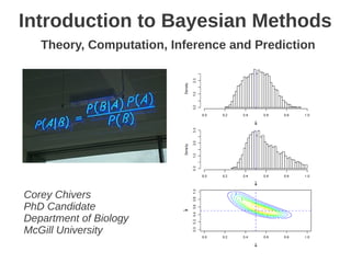
Introduction to Bayesian Methods
•
63 gostaram•17,302 visualizações

This document provides an introduction to Bayesian methods for theory, computation, inference and prediction. It discusses key concepts in Bayesian statistics including the likelihood principle, the likelihood function, Bayes' theorem, and using Markov chain Monte Carlo methods like the Metropolis-Hastings algorithm to perform posterior integration when closed-form solutions are not possible. Examples are provided on using Bayesian regression to model the relationship between salmon body length and egg mass while incorporating prior information. The summary concludes that the Bayesian approach provides a coherent way to quantify uncertainty and make predictions accounting for both aleatory and epistemic sources of variation.

Recomendados
Mais conteúdo relacionado
Mais procurados
Mais procurados (20)
Semelhante a Introduction to Bayesian Methods
Semelhante a Introduction to Bayesian Methods (14)
Último
Último (20)
Introduction to Bayesian Methods
- 1. Introduction to Bayesian Methods Theory, Computation, Inference and Prediction Corey Chivers PhD Candidate Department of Biology McGill University
- 2. Script to run examples in these slides can be found here: bit.ly/Wnmb2W These slides are here: bit.ly/P9Xa9G
- 5. The Likelihood Principle ● All information contained in data x, with respect to inference about the value of θ, is contained in the likelihood function: L | x ∝ P X= x | Corey Chivers, 2012
- 6. The Likelihood Principle L.J. Savage R.A. Fisher Corey Chivers, 2012
- 7. The Likelihood Function L | x ∝ P X= x | L | x =f | x Where θ is(are) our parameter(s) of interest ex: Attack rate Fitness Mean body mass Mortality etc... Corey Chivers, 2012
- 8. The Ecologist's Quarter Lands tails (caribou up) 60% of the time Corey Chivers, 2012
- 9. The Ecologist's Quarter Lands tails (caribou up) 60% of the time ● 1) What is the probability that I will flip tails, given that I am flipping an ecologist's quarter (p(tail=0.6))? P x | =0.6 ● 2) What is the likelihood that I am flipping an ecologist's quarter, given the flip(s) that I have observed? L=0.6 | x Corey Chivers, 2012
- 10. The Ecologist's Quarter T H L | x = ∏ ∏ 1− t=1 h=1 L=0.6 | x=H T T H T 3 2 = ∏ 0.6 ∏ 0.4 t =1 h=1 = 0.03456 Corey Chivers, 2012
- 11. The Ecologist's Quarter T H L | x = ∏ ∏ 1− t=1 h=1 L=0.6 | x=H T T H T 3 2 But what does this = ∏ 0.6 ∏ 0.4 mean? 0.03456 ≠ P(θ|x) !!!! t =1 h=1 = 0.03456 Corey Chivers, 2012
- 12. How do we ask Statistical Questions? A Frequentist asks: What is the probability of having observed data at least as extreme as my data if the null hypothesis is true? P(data | H0) ? ← note: P=1 does not mean P(H0)=1 A Bayesian asks: What is the probability of hypotheses given that I have observed my data? P(H | data) ? ← note: here H denotes the space of all possible hypotheses Corey Chivers, 2012
- 13. P(data | H0) P(H | data) But we both want to make inferences about our hypotheses, not the data. Corey Chivers, 2012
- 14. Bayes Theorem ● The posterior probability of θ, given our observation (x) is proportional to the likelihood times the prior probability of θ. P x | P P | x= P x Corey Chivers, 2012
- 15. The Ecologist's Quarter Redux Lands tails (caribou up) 60% of the time Corey Chivers, 2012
- 16. The Ecologist's Quarter T H L | x = ∏ ∏ 1− t=1 h=1 L=0.6 | x=H T T H T 3 2 = ∏ 0.6 ∏ 0.4 t =1 h=1 = 0.03456 Corey Chivers, 2012
- 17. Likelihood of data given hypothesis P( x | θ) But we want to know P(θ | x ) Corey Chivers, 2012
- 18. ● How can we make inferences about our ecologist's quarter using Bayes? P( x | θ) P(θ) P(θ | x )= P( x ) Corey Chivers, 2012
- 19. ● How can we make inferences about our ecologist's quarter using Bayes? Likelihood P x | P P | x= P x Corey Chivers, 2012
- 20. ● How can we make inferences about our ecologist's quarter using Bayes? Likelihood Prior P( x | θ) P(θ) P(θ | x )= P( x ) Corey Chivers, 2012
- 21. ● How can we make inferences about our ecologist's quarter using Bayes? Likelihood Prior P x | P P | x= Posterior P x Corey Chivers, 2012
- 22. ● How can we make inferences about our ecologist's quarter using Bayes? Likelihood Prior P x | P P | x= Posterior P x P x =∫ P x | P d Not always a closed form solution possible!! Corey Chivers, 2012
- 24. Randomization to Solve Difficult Problems ` Feynman, Ulam & Von Neumann ∫ f d Corey Chivers, 2012
- 25. Monte Carlo Throw darts at random Feynman, Ulam & Von Neumann (0,1) P(blue) = ? P(blue) = 1/2 P(blue) ~ 7/15 ~ 1/2 (0.5,0) (1,0) Corey Chivers, 2012
- 26. Your turn... Let's use Monte Carlo to estimate π - Generate random x and y values using the number sheet - Plot those points on your graph How many of the points fall within the circle? y=17 x=4
- 27. Your turn... Estimate π using the formula: ≈4 # in circle / total
- 28. Now using a more powerful computer!
- 29. Posterior Integration via Markov Chain Monte Carlo A Markov Chain is a mathematical construct where given the present, the past and the future are independent. “Where I decide to go next depends not on where I have been, or where I may go in the future – but only on where I am right now.” -Andrey Markov (maybe) Corey Chivers, 2012
- 32. Metropolis-Hastings Algorithm 1. Pick a starting location at The Markovian Explorer! random. 2. Choose a new location in your vicinity. 3. Go to the new location with probability: p=min 1, x proposal x current 4. Otherwise stay where you are. 5. Repeat. Corey Chivers, 2012
- 33. MCMC in Action! Corey Chivers, 2012
- 34. ● We've solved our integration problem! P x | P P | x= P x P | x∝ P x | P Corey Chivers, 2012
- 35. Ex: Bayesian Regression ● Regression coefficients are traditionally estimated via maximum likelihood. ● To obtain full posterior distributions, we can view the regression problem from a Bayesian perspective. Corey Chivers, 2012
- 36. ##@ 2.1 @## Corey Chivers, 2012
- 37. Example: Salmon Regression Model Priors Y =a+ bX +ϵ a ~ Normal (0,100) ϵ ~ Normal( 0, σ) b ~ Normal (0,100) σ ~ gamma (1,1/ 100) P( a , b , σ | X , Y )∝ P( X ,Y | a , b , σ) P( a) P(b) P( σ) Corey Chivers, 2012
- 38. Example: Salmon Regression Likelihood of the data (x,y), given the parameters (a,b,σ): n P( X ,Y | a , b , σ)= ∏ N ( y i ,μ=a+ b x i , sd=σ) i=1 Corey Chivers, 2012
- 42. ##@ 2.5 @## >## Print the Bayesian Credible Intervals > BCI(mcmc_salmon) 0.025 0.975 post_mean a -13.16485 14.84092 0.9762583 b 0.127730 0.455046 0.2911597 Sigma 1.736082 3.186122 2.3303188 Inference: Does body length have EM =ab BL an effect on egg mass? Corey Chivers, 2012
- 43. The Prior revisited ● What if we do have prior information? ● You have done a literature search and find that a previous study on the same salmon population found a slope of 0.6mg/cm (SE=0.1), and an intercept of -3.1mg (SE=1.2). How does this prior information change your analysis? Corey Chivers, 2012
- 45. Example: Salmon Regression Informative Model Priors EM =ab BL a ~ Normal (−3.1,1 .2) ~ Normal 0, b ~ Normal (0.6,0 .1) ~ gamma1,1 /100 Corey Chivers, 2012
- 46. If you can formulate the likelihood function, you can estimate the posterior, and we have a coherent way to incorporate prior information. Most experiments do happen in a vacuum. Corey Chivers, 2012
- 47. Making predictions using point estimates can be a dangerous endeavor – using the posterior (aka predictive) distribution allows us to take full account of uncertainty. How sure are we about our predictions? Corey Chivers, 2012
- 48. Aleatory Stochasticity, randomness Epistemic Incomplete knowledge
- 49. ##@ 3.1 @## ● Suppose you have a 90cm long individual salmon, what do you predict to be the egg mass produced by this individual? ● What is the posterior probability that the egg mass produced will be greater than 35mg? Corey Chivers, 2012
- 51. P(EM>35mg | θ) Corey Chivers, 2012
- 52. Extensions: Clark (2005)
- 53. Extensions: ● By quantifying our uncertainty through integration of the posterior distribution, we can make better informed decisions. ● Bayesian analysis provides the basis for decision theory. ● Bayesian analysis allows us to construct hierarchical models of arbitrary complexity. Corey Chivers, 2012
- 54. Summary ● The output of a Bayesian analysis is not a single estimate of θ, but rather the entire posterior distribution., which represents our degree of belief about the value of θ. ● To get a posterior distribution, we need to specify our prior belief about θ. ● Complex Bayesian models can be estimated using MCMC. ● The posterior can be used to make both inference about θ, and quantitative predictions with proper accounting of uncertainty. Corey Chivers, 2012
- 55. Questions for Corey ● You can email me! Corey.chivers@mail.mcgill.ca ● I blog about statistics: bayesianbiologist.com ● I tweet about statistics: @cjbayesian
- 56. Resources ● Bayesian Updating using Gibbs Sampling http://www.mrc-bsu.cam.ac.uk/bugs/winbugs/ ● Just Another Gibbs Sampler http://www-ice.iarc.fr/~martyn/software/jags/ ● Chi-squared example, done Bayesian: http://madere.biol.mcgill.ca/cchivers/biol373/chi- squared_done_bayesian.pdf Corey Chivers, 2012