Digital image processing ,Techniques of Digital Image Processing Image Enhancement ,Image Histogram,Spatial Filtering,Smoothing and Sharpening Examples,Image Classification,Supervised Classification,Unsupervised Classification remote sensing applications.

2. UNIT III
Digital image processing (DIP)
It is the task of processing and analyzing the digital data using some image
processing algorithm. The analysis of relies only upon multispectral characteristic
of the feature represented in the form of tone and color.
Most of the common image processing functions available in image analysis
systems can be categorized into the following four categories:
1. Preprocessing (Image rectification and restoration)
2. Image Enhancement
3. Image Classification and Analysis
4. Data Merging and GIS Interpretation

3. Techniques of Digital Image Processing
Initial Data Statistics
Statistical information such as minimum and maximum values of the data set, mean, standard
deviation, and variance for each band are calculated. Histograms and scatter-grams provide a
graphical view of the nature of different bands.
Image Rectification and Restoration ( or Preprocessing)
These are correction needed for the distortion or degradations of raw data. Radiometric and
geometric correction are applicable to this.
Image Enhancement
Purpose of this is to improve the appearance of the imaginary and to assist in subsequent
visual interpretation and analysis. Normally, image enhancement involves techniques for
increasing the visual distinction between features by improving tonal distinction between
various features in a sene using technique of contrast stretching.
Image Transformation
These are operations similar in concept to image enhancement. Generally, image
enhancement operation is carried out on a single band of data, while image transformations
are usually on multiple bands.
Image Classification
The objective of the classification is to replace visual analysis of the image data with
quantitative techniques for automating the identification of features in a scene.

4. Digital Data
Initial Display of Image
Initial Statistic Extraction
Image Rectification and Restoration
Image Enhancement
Visual Analysis
Image Classification
Ancillary Data
Unsupervised
Supervised
Classified Output
Post processing operation
Data Merging
Assessment of Accuracy
Maps and Images
Report
Data

5. Image Enhancement
(Histogram Example)
Original

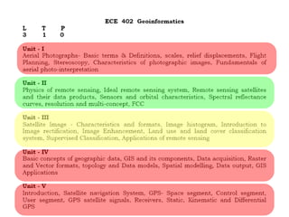
6. Histogram Example (cont. )
Poor contrast

7. Histogram Example (cont. )
Poor contrast

8. Histogram Example (cont. )
Enhanced contrast

9. Image Histogram
An image histogram is a
graphical representation of the
brightness values that
comprise an image. The
brightness values (i.e. 0-255)
are displayed along the x-axis
of the graph and the frequency
of occurrence of each of these
values in the image on the Yaxis. By manipulating the
range of digital values in an
image, i.e. graphically
represented by its histogram,
various enhancement can be
applied to the data. However,
these can be grouped under
two categories:
1.
Linear contrast Enhancement
2.
Non linear contrast
Enhancement

10. Spatial Filtering
Spatial filtering is the digital processing function that are used to enhance the
appearance of an image. Spatial features are designed to highlight or suppress
specific features in an image based on their spatial frequency.
Spatial frequency is related to the concept of image texture. It refers to the
frequency of the variations in tone that appear in an image. Rough texture areas of
an image, where the changes in tone are abrupt over a small area, have high
spatial frequencies, while smooth areas with little variation in tone over several
pixels, have low spatial frequencies.
Types of Filters
1. Low-pass Filter: is designed to emphasize large homogenous areas of
similar tone and reduce the smaller detail in an image. Thus, these filters generally
serve to smooth the appearance of an image.
2. High-pass Filter: such filters do the opposite job as low-pass filter. They are
served to sharpen the appearance of fine details in an image.
Other Filters
1. High boost filters
2. Directional or edge detection filters

11. Smoothing and Sharpening Examples
Smoothing
(Low-pass Filter)
Sharpening
(High-pass Filter)

12. Image Classification
Purpose
•
To identify and map areas with similar characteristics
•
To assign meaningful categories such as land-use or land-cover classes
to pixel values
Classification Methods
1. Supervised classification
2. Unsupervised classification

13. Supervised Classification
In this classification method, an analyst identifies the imaginary in terms of
homogenous representative samples of different surface cover type of
interest. These samples are called as “Training Areas”.
The selection of appropriate training area is based on the analyst’s familiarity
with geographical area and knowledge of the actual surface cover types
present in the image.
The numerical information in all spectral bands for the pixels comprising these
areas are used to train the computer to recognize specially similar areas for
each class.
Therefore, in supervised classification, the analyst is first identifies the
information classes based on which it determines the spectral classes which
represent them.
Common Classifiers:
1. Parallel-piped classifiers
2. Minimum distance to mean classifiers
3. Maximum likelihood classifiers (MLC)

14. Supervised Classification
Supervised classification requires the
analyst to select training areas where
he/she knows what is on the ground
and then digitize a polygon within that
area…
The computer then creates...
Mean Spectral
Signatures
Conifer
Known Conifer
Area
Water
Known Water
Areac
Deciduous
Known Deciduous
Area
Digital Image

15. Supervised Classification
Mean Spectral
Signatures
Multispectral Image
Information
(Classified Image)
Conifer
Deciduous
Water
Unknown
Spectral Signature
of Next Pixel to be
Classified

16. Unsupervised Classification
Unsupervised classification reverses the supervised classification process.
Spectral classes are grouped first, based only on the numerical information in
the data and are then matched by the analyst to information classes.
Programs called Clustering algorithms are used to determine the natural
groupings or structures in the data. Usually, the analyst specify how many
groups or clusters are to be looked for in the data.
In addition to specifying the desired number of classes, the analyst may also
specify the parameters related to separation distance among the clusters and
variation with each cluster
However, algorithm for this classification operates in a two- pass mode. In the
first pass, the algorithm sequentially builds class clusters. In second pass, a
minimum distance classifier is applied to the whole data set on a pixel-by-pixel
basis, where each pixel is assigned to one of the mean vectors created in pass
1 mode.

17. Unsupervised Classification
The analyst requests the computer to examine
the image and extract a number of spectrally
distinct clusters…
Spectrally Distinct Clusters
Cluster 3
Cluster 5
Cluster 1
Digital Image
Cluster 6
Cluster 2
Cluster 4

18. Unsupervised Classification
Saved Clusters
Cluster 3
Cluster 5
Cluster 1
Output Classified Image
Cluster 6
Cluster 2
Next Pixel to
be Classified
Cluster 4
Unknown

19. Unsupervised Classification
The result of the
unsupervised classification is
not yet information until…
The analyst determines the
ground cover for each of the
clusters…
???
Water
???
Water
???
Conifer
???
Conifer
???
Hardwood
???
Hardwood

20. Remote Sensing Applications
Land Use/Land Cover mapping
1. Natural resource management
2. Wildlife protection
3. Encroachment
Urban Planning
Forestry & Ecosystem
1. Land parcel mapping
1. Forest cover & density mapping
2. Infrastructure mapping
2. Deforestation mapping
3. Land use change detection
3. Forest fire mapping
4. Future urban expansion planning
4. Wetland mapping and monitoring
Agriculture
1. Crop type classification
2. Crop condition assessment
3. Crop yield estimation
4. Mapping of soil characteristic
5. Soil moisture estimation
5. Biomass estimation
6. Species inventory

21. Remote Sensing Applications
……cont.
Geology
1. Lithological mapping
2. Mineral exploration
3. Environmental geology
Hydrology
4. Sedimentation mapping and monitoring
1. Watershed mapping & management
5. Geo-hazard mapping
2. Flood delineation and mapping
6. Glacier mapping
3. Ground water targeting
Ocean applications
1. Storm forecasting
Other Applications
2. Water quality monitoring
1. Flood Plain Mapping
3. Aquaculture inventory and monitoring
2. Disaster Management
4. Navigation routing
3. District level Planning
5. Coastal vegetation mapping
6. Oil spill

22. Land Use And Land Cover Mapping
A study on land use and land cover for a part of
Hraidwar district was carried out for the area lying
LISS III PAN
between 78007’13” E and 78016’14” E longitude and
300 N and 30008’53” N latitudes covering an area of
Initial Statistics
nearly 260 km2.
IRS-1C LISS III of April 3, 2000 was used along with
Contrast Enhancement
PAN image of the same date. The methodology
adopted is shown in figure.
Registration
On the basis of field visit, 11 cities
were identified. These classes are:
i). Thin forest
ii). Medium forest
iii). Dense forest
vi). Open land
Supervised Classification
iv). Fallow land
v). Shrubs
Ground Data
Classified Image
vii). Shallow water viii). Wet land
ix). Dry sand
xi). Deep water
x). Built-up-area
Accuracy Assessment