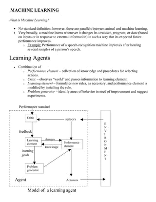
1. MACHINE LEARNING
What is Machine Learning?
• No standard definition, however, there are parallels between animal and machine learning.
• Very broadly, a machine learns whenever it changes its structure, program, or data (based
on inputs or in response to external information) in such a way that its expected future
performance improves.
o Example: Performance of a speech-recognition machine improves after hearing
several samples of a person’s speech.
Learning Agents
• Combination of
o Performance element – collection of knowledge and procedures for selecting
actions.
o Critic – observes “world” and passes information to learning element.
o Learning element – formulates new rules, as necessary, and performance element is
modified by installing the rule.
o Problem generator – identify areas of behavior in need of improvement and suggest
experiments.
Performance standard
Critic sensors
E
N
feedback V
I
R
Learning changes
Performance O
element N
knowledge element
M
learning E
goals N
T
Problem
generator
Agent Actuators
Model of a learning agent

2. DECISION TREES
Motivation
o When a businessperson needs to make a decision based on several factors, a decision tree
can help identify which factors to consider and how each factor has historically been
associated with different outcomes of the decision.
o For example, in a credit risk case study, we have data for each applicant’s debt, income,
and marital status.
o A decision tree creates a model as either a graphical tree or a set of text rules that can
predict (classify) each applicant as a good or bad credit risk.
A decision tree is a model that is both predictive and descriptive. It is called a decision tree
because the resulting model is presented in the form of a tree structure.
o Visual presentation makes the decision tree model very easy to understand and assimilate.
Decision trees are most commonly used for classification (predicting what group a case
belongs to), but can also be used for regression (predicting a specific value).
o Decision trees graphically display the relationships found in data. It shows the relationship
between one dependent variable (e.g. credit risk) and several independent variables (e.g.
income, debt, and marital status).
o A goal in a decision tree is of the form G ⇔ P1 ∨ P2 ∨ …. ∨ Pn, where each Pi is a
conjunction of tests from the root of the tree to a leaf with a positive outcome.
o Most products also translate the tree-to-text rules such as If Income = High and Years on
job > 5 Then Credit risk = Good.
o Decision tree algorithms are very similar to rule induction algorithms which produce rule
sets without a decision tree.
o The training process that creates the decision tree is usually called induction.

3. Example : The credit risk classification problem
Name Debt Income Married? Risk
Joe 1 1 1 1
Sue 0 1 1 1
John 0 1 0 0
Mary 1 0 1 0
Fred 0 0 1 0
Credit risk data with column values converted to numeric values.
Predicted
High Not
Risk Low Debt High Income Low Income Married
Debt Married
Good 1 1 2 0 2 0
Poor 1 2 1 2 2 1
Cross-tabulation of the independent vs. dependent columns for the root node.
The resulting tree is:
Note:
o Each box in the tree represents a node.
o The tree grows from the root node – the
data is split at each level to form new
nodes.
o The leaf nodes play a special role when
the tree is used for prediction

4. Note the following:
o In the tree, each node contains information about the number of instances at that node, and
about the distribution of dependent variable values (Credit Risk).
o The instances at the root node are all of the instances in the training set - instances, of
which 40 percent are Good risks and 60 percent are Poor risks.
o Below the root node (parent) is the first split that, in this case, splits the data into two new
nodes (children) based on whether Income is High or Low.
o The rightmost node (Low Income) resulting from this split contains two instances,
both of which are associated with Poor credit risk.
 Because all instances have the same value of the dependent variable (Credit
Risk), this node is termed pure and will not be split further.
o The leftmost node in the first split contains three instances, 66.7 % of which are
Good.
o The leftmost node is then further split based on the value of Married (Yes or No),
resulting in two more nodes which are each also pure.
Note also
 The order of the splits, Income first and then Married, is determined by an induction
algorithm - the method used in the above tree is to pick the split that has the largest
number of instances on the diagonal of its cross-tabulation.
 Once grown, a tree can be used for predicting a new case by starting at the root (top) of the
tree and following a path down the branches until a leaf node is encountered. The path is
determined by imposing the split rules on the values of the independent variables in the
new instance.
Example
Consider the first row in the training set for Joe. Because Joe has High income, follow the branch
to the left. Because Joe is married, follow the tree down the branch to the right. At this point we
have arrived at a leaf node, and the predicted value is the predominant value of the leaf node, or
Good in this case.
The rules for the leaf nodes, taken left to right, are as follows:
IF Income = High AND Married = No THEN Risk = Poor
IF Income = High AND Married = Yes THEN Risk = Good
IF Income = Low THEN Risk = Poor
There are often additional interesting and potentially useful observations about the data that can
be made after a tree has been induced. In the case of our sample data, the tree reveals:
• Debt appears to have no role in determining Risk.
• People with Low Income are always a Poor Risk.

5. • Income is the most significant factor in determining risk.