
Recomendados
Mais conteúdo relacionado
Mais procurados
Mais procurados (20)
Destaque
Semelhante a Price and performance in funds gil bazo
Semelhante a Price and performance in funds gil bazo (20)
Mais de bfmresearch
Mais de bfmresearch (20)
Último
Último (20)
Price and performance in funds gil bazo
- 1. THE JOURNAL OF FINANCE • VOL. LXIV, NO. 5 • OCTOBER 2009 The Relation between Price and Performance in the Mutual Fund Industry JAVIER GIL-BAZO and PABLO RUIZ-VERDU∗ ´ ABSTRACT Gruber (1996) drew attention to the puzzle that investors buy actively managed equity mutual funds, even though on average such funds underperform index funds. We uncover another puzzling fact about the market for equity mutual funds: Funds with worse before-fee performance charge higher fees. This negative relation between fees and performance is robust and can be explained as the outcome of strategic fee-setting by mutual funds in the presence of investors with different degrees of sensitivity to performance. We also find some evidence that better fund governance may bring fees more in line with performance. MANY STUDIES HAVE attempted to determine whether equity mutual funds are able to consistently earn positive risk-adjusted returns.1 Although these studies have documented significant differences in risk-adjusted returns across funds, it became apparent early on (Sharpe (1966)) that those differences are to a large extent attributable to differences in fund fees. Most research on mutual funds has thus been aimed at determining whether the cross-sectional variation in performance that is not explained by fees can be explained by the existence of managers with superior stock-picking skills (see, e.g., Chevalier and Ellison (1999)). However, little attention has been paid to the relation between before- fee performance and fees. In this paper, we focus on this relation and investigate whether differences in fees ref lect differences in the value that mutual funds create for investors. ∗ Gil-Bazo and Ruiz-Verdu are with the Department of Business Administration, Universidad ´ Carlos III de Madrid. The authors thank Campbell Harvey (the editor), an anonymous associate editor, and an anonymous referee for their comments, which have led to substantial improvements in the paper. We are also grateful to Laurent Barras, Clemens Sialm, Massimo Guidolin, Alfonso ¨e Novales, Mikel Tapia, Manuel F. Bagu´ s, Fr´ d´ ric Warzynski, and Ralph Koijen as well as sem- e e inar participants at Tilburg University, IE Business School, University of the Basque Country, Universidad de Navarra, Universitat Pompeu Fabra, Universidad Carlos III de Madrid, Financial Management Association European Conference, and the annual meeting of the European Financial Management Association for helpful comments and suggestions. The usual disclaimer applies. Part of the paper was written while Javier Gil-Bazo was visiting the Finance Department of Tilburg University. The financial support of Spain’s Ministry of Education and Science (SEJ2005-06655, SEJ2007-67448, and Consolider-Ingenio CSD2006-16), the BBVA Foundation, and the Madrid Au- tonomous Region (CCG07-UC3M/HUM-3413) is gratefully acknowledged. 1 See, for example, Brown and Goetzmann (1995); Gruber (1996); Carhart (1997); Daniel et al. (1997); Wermers (2000); Cohen, Coval, and Pastor (2005); Kacperczyk, Sialm, and Zheng (2005); or Kosowski et al. (2006). 2153
- 2. 2154 The Journal of Finance R Mutual fund fees pay for the services provided to investors by the fund. Be- cause the main service provided by a mutual fund is portfolio management, fees should ref lect funds’ risk-adjusted performance. It follows that there should be a positive relation between before-fee risk-adjusted expected returns and fees. In contrast to this prediction, we find a puzzling negative relation between before- fee risk-adjusted performance and fees in a sample of U.S. equity mutual funds: Funds with worse before-fee risk-adjusted performance charge higher fees. To check the robustness of this finding, we use different estimation methods and performance measures, and we investigate the relation for different subsam- ples. The negative relation between before-fee risk-adjusted performance and fees survives these robustness checks. We then set out to explain this anomalous relation by investigating the role of performance in the determination of fund fees. Christoffersen and Musto (2002) propose that mutual funds’ fees are set taking into account the elasticity of the demand for their shares, so that funds facing less elastic demand charge higher fees. These authors argue that funds with worse past performance face less elastic demand because performance-sensitive investors leave funds fol- lowing bad performance. If performance is persistent for at least the worse- performing funds (as indicated by Carhart (1997)), Christoffersen and Musto’s hypothesis could explain our finding of a negative relation between fees and ´ before-fee performance. Gil-Bazo and Ruiz-Verdu (2008) provide a related ex- planation. These authors set forth a model of the market for mutual funds in which competition among high-performance funds for the money of sophisti- cated (performance-sensitive) investors pushes their fees down and drives the low-performance funds out of that segment of the market. Low-performance funds then target unsophisticated investors, to whom they are able to charge higher fees. We also consider the possibility that funds with low expected per- formance have higher fees because they incur higher marketing costs, which they pass on to investors. Underperforming funds will have high distribution costs or advertising outlays if they target unsophisticated investors, and these investors are more responsive to advertising or more likely to use brokers to purchase mutual funds. We test these strategic fee-setting hypotheses against an alternative cost-based explanation, according to which the negative relation between performance and fees that results from univariate regressions would simply be due to the omission of fund characteristics associated with both lower operating costs and better performance. To test these hypotheses, we estimate the relation between fund fees and performance, investors’ sensitivity to fund performance, which we measure by the estimated slope of the relation between performance and money f lows, and a number of variables that have been previously identified as determinants of funds’ operating costs. Our results are consistent with the strategic explana- tions described earlier: Even after controlling for a host of fund characteris- tics, underperforming funds and funds faced with less performance-sensitive investors charge higher marketing and nonmarketing fees. The apparent inability of mutual fund competition to ensure an adequate relation between risk-adjusted performance and fees raises the question of
- 3. Price and Performance in the Mutual Fund Industry 2155 whether improvements in mutual fund governance can bring fees more into line with the value that funds generate for investors. To evaluate the poten- tial effects of recent regulatory reforms that impose stricter requirements on mutual fund governance, we analyze the role played by fund governance in fee determination. We find some evidence that funds with boards of directors expected, a priori, to provide more effective protection of investors’ interests charge fees that better ref lect their risk-adjusted performance. The paper is organized as follows. In Section I, we describe the mutual fund fee structure and the data set. In Section II, we explain how we estimate fund performance. In Section III, we estimate the relation between before-fee per- formance and fees and perform several tests to evaluate the robustness of the results. In Section IV, we discuss and test several explanations for the esti- mated relation between fees and performance. Section V concludes. I. Data A. Mutual Fund Fee Structure Fund management fees are typically computed as a fixed percentage of the value of assets under management.2 These fees, together with other operating costs, such as custodian, administration, accounting, registration, and transfer agent fees—comprise the fund’s expenses, which are deducted on a daily basis from the fund’s net assets by the managing company. Expenses are usually expressed as a percentage of assets under management known as the “expense ratio.” Fees paid to brokers in the course of the fund’s trading activity are detracted from the fund’s assets, but are not included in the expense ratio. Funds often charge “loads,” which are one-time fees that are used to pay distributors. These loads are paid at the time of purchasing (“front-end load”) or redeeming (“back-end load” or “deferred sales charge”) fund shares and are computed as a fraction of the amount invested.3 Since 1980, funds may charge so-called “12b-1 fees,” which are included in the expense ratio and, like loads, are used to pay for marketing and distribution costs. Since the 1990s, many funds offer multiple share classes with different combinations of loads and 12b-1 fees. Among the most common classes are class A shares, which are characterized by high front-end loads and low annual 12b-1 fees, and class B and C shares, which typically have no or low front-end loads but have higher 12b-1 fees and a contingent deferred sales load. This contingent deferred sales load decreases the longer the shares are held and is eventually eliminated (typically after 1 year for class C shares, and after 6 to 7 years for class B shares). 2 Some funds allow the percentage to depend on fund performance. Although our data do not allow us to identify these funds, the evidence reported in Elton, Gruber, and Blake (2003), Kuhnen (2005), and Warner and Wu (2006) suggests that for most of our sample period the fraction of funds with incentive fees is very small. 3 Funds often waive at least a fraction of the loads. Therefore, the loads typically reported in databases, such as the one we use in this paper, can often overestimate effective loads.
- 4. 2156 The Journal of Finance R B. Sample Description We obtain our data from the Center for Research in Security Prices (CRSP) Survivor-Bias Free U.S. Mutual Fund Database for the period from December 1961 to December 2005 (see Carhart (1997), Elton, Gruber, and Blake (2001), and Carhart et al. (2002) for detailed discussions of the data set). The initial sample contains all open-end mutual funds that are active in the 1961 to 2005 period. From this initial sample, we exclude all funds that we cannot confi- dently describe as diversified domestic equity mutual funds. Thus, we remove money market, bond and income, and specialty mutual funds, such as sector or international funds. To obtain our sample of diversified domestic equity mutual funds, we use the information on funds’ investment objectives available in the CRSP database. Unfortunately, this information is not consistent throughout the 1961 to 2005 period. To create a homogeneous sample for the full sample pe- riod, we combine all the information available on funds’ investment objectives. Some of our results, however, are derived only for the 1992 to 2005 period, for which the information on funds’ investment objectives is precise and consistent. We remove from the sample observations with no information on returns or expenses, or with zero expenses. The remaining sample contains some ob- servations with extreme values for expenses or returns that are either data errors, or that correspond to small funds with unusually high expenses or very high volatility. Given the large size of the data set, we use Hadi’s (1994) out- lier detection method to search for these outliers and remove them from the sample. Finally, to ensure that our results are not driven by differences between index and actively managed funds or between institutional and retail funds, we iden- tify passively managed (index) and institutional funds and exclude them from the sample. In the Internet Appendix,4 we provide a more detailed account of the procedure we use to construct our final sample, as well as summary statis- tics of the main variables. C. Fund Governance Data We use the January 2007 Morningstar Principia CD to obtain data on mu- tual funds’ board quality. This data set includes several governance ratings as of December 2006, which Morningstar uses to compute the so-called “Steward- ship Grade” for mutual funds. The measure of board quality that we use in our analysis (Morningstar’s “board quality” grade) is the sum of four equally weighted components that measure, respectively, the degree to which the board has taken action “in cases where the fund clearly has not served investors well”; the significance of independent directors’ investments in the fund; whether the board is “overseeing so many funds that it may compromise the ability to dili- gently protect the interests of shareholders”; and whether the fund meets the Securities and Exchange Commission (SEC) requirement for the proportion of 4 The Internet Appendix is available at http://www.afajof.org/supplements.asp.
- 5. Price and Performance in the Mutual Fund Industry 2157 Table I Summary Statistics: Board Quality Measure The table shows the distribution of the board quality grade provided by Morningstar for funds in the governance subsample in year 2005. The first row reports the frequency of each grade; the second row reports the relative frequency (in percentage terms); and the third row reports the cumulative frequency (in percentage terms). Very Poor Poor Fair Good Excellent Total Frequency 1 69 374 486 176 1,106 % 0.09 6.24 33.82 43.94 15.91 100 Cumulative 0.09 6.33 40.14 84.09 100 independent directors, regardless of whether it is subject to the requirement (see Morningstar (2006), pp. 1–2, for a detailed description). Thus, the board quality grade is closely related to board characteristics that have been the focus of both regulatory reform and academic research.5 Of the 3,677 actively managed, diversified, noninstitutional funds (fund classes) that are active in 2005 in our sample, there is board quality infor- mation in Morningstar’s January 2007 Principia CD for only 1,106 funds (the governance subsample). Although only one-third of the funds in the sample be- long to the governance subsample, these funds manage almost 80% of the total net assets managed by all funds in the sample. We note that the governance subsample is not a random sample from the whole population. Among other differences, funds in the governance subsample perform significantly better on average, belong to larger management companies, and are cheaper, larger, and older than those in the nongovernance subsample. Table I reports the distribution of board quality grades. There are five grades to which Morningstar assigns a numerical score that ranges from zero to two: Very Poor (0), Poor (0.5), Fair (1), Good (1.5), and Excellent (2). As Table I shows, most funds have Fair or Good grades, and only one obtains a Very Poor grade. The resulting average grade lies between Fair and Good. II. Mutual Fund Performance Estimation We use Carhart’s (1997) four-factor model to estimate before-fee risk-adjusted performance: rit = αi + βrm,i rmt + βsmb,i smbt + βhml,i hmlt + βpr1 y,i pr1yt + εit , (1) where rit is fund i’s before-expense return in month t in excess of the 30-day risk- free interest rate—proxied by Ibbotson’s 1-month Treasury bill rate;6 rmt is the 5 Morningstar’s Stewardship Grade includes other components. See Wellman and Zhou (2008) for a recent analysis of the Morningstar Stewardship Grade. 6 Because fund returns are reported after expenses, to retrieve monthly before-expense returns, we add annual expenses divided by 12 to reported returns. This measure is only an approximation
- 6. 2158 The Journal of Finance R market portfolio return in excess of the risk-free rate; and smbt and hmlt denote the return on portfolios that proxy for common risk factors associated with size and book-to-market, respectively. The term pr1yt is the return difference between stocks with high and low returns in the previous year. We include this term to account for passive momentum strategies by mutual funds.7 The term αi is the fund’s alpha and captures the fund’s before-fee risk-adjusted performance. We also consider Fama and French’s (1993) three-factor model, which uses only rmt , smbt , and hmlt , as well as conditional versions of the four- factor model. As in Carhart (1997), we follow a two-stage estimation procedure to obtain a panel of monthly fund risk-adjusted performance estimates. In the first stage, for every month t in years 1967 to 2005, we regress funds’ before-fee excess returns on the risk factors over the previous 5 years. If less than 5 years of previous data are available for a specific fund-month, we require the fund to be in the sample for at least 48 months in the previous 5 years, and then run the regression with the available data. In the second stage, we estimate a fund’s risk-adjusted performance in month t as the difference between the fund’s before-expense excess return and the realized risk premium, defined as the vector of betas times the vector of factor realizations in month t.8 Rolling regressions yield a total of 232,386 monthly risk-adjusted before-fee returns corresponding to 3,109 different actively managed retail funds over 468 months. Although the average annualized monthly return before expenses in our sample equals 10.52%, subtracting the risk-free rate and the part of fund returns explained by the portfolio’s exposure to the Fama–French three factors yields an average annualized monthly alpha of −21 basis points (bp), which is further reduced to −70.6 bp when we take momentum into account. The corresponding annualized standard deviations are 18.13%, 7.33%, and 7.15%, respectively. III. The Relation between Fees and Performance In a well-functioning mutual fund market, mutual fund fees should be posi- tively correlated with expected before-fee risk-adjusted returns. Further, in the absence of market frictions, all funds should earn zero expected after-fee risk- adjusted returns in equilibrium since, otherwise, there would be excess demand (supply) for funds with positive (negative) expected after-fee risk-adjusted re- turns (Berk and Green (2004)). In this context, if investors know funds’ alphas, because we ignore the compounding effect of the accrual of expenses over the year, and because the actual accrual of expenses may not be completely smooth (Tufano, Quinn, and Taliaferro (2006)). 7 Data are downloaded from Kenneth French’s web site, http://mba.tuck.dartmouth.edu/pages/ faculty/ken.french/. 8 We follow Fama and MacBeth (1973) in our choice of a 5-year estimation period, instead of the 3-year period used by Carhart (1997). Although a longer estimation period excludes a greater fraction of funds from the sample, it also reduces sampling error in betas and mitigates the effect of two forms of selection bias that affect mostly the subset of young funds in the CRSP database: omission bias and incubation bias (Elton, Gruber, and Blake (2001) and Evans (2009)).
- 7. Price and Performance in the Mutual Fund Industry 2159 then equilibrium requires that αi − fi = 0 for every fund i, where fi denotes fund i’s fees, expressed as a fraction of the fund’s assets. This equilibrium condition can be equivalently written as αi = fi , for every fund i. Therefore, a graph depict- ing the equilibrium relation between fees and before-fee performance should yield an increasing linear relation with a slope of one. If, on the other hand, investors do not know funds’ alphas, then αi in the equilibrium condition is replaced by investors’ expectation of fund i’s risk-adjusted returns. Equilibrium in the mutual fund market can be achieved through fee adjust- ment if funds with higher expected before-fee risk-adjusted returns increase their fees or underperforming funds lower theirs. However, Berk and Green (2004) show that in the market for mutual funds, market clearing can also be achieved via quantity adjustment: If there are decreasing returns to scale in fund management, then f lows of money into funds that are expected to perform better will reduce those funds’ expected performance until expected after-fee risk-adjusted returns are equalized across all funds in equilibrium. Whether market clearing takes place via fees, quantities, or a combination of both is, however, not material for the definition of market equilibrium. In any case, equilibrium requires that expected after-fee risk-adjusted returns be zero for all funds, and thus implies the linear relation (with a slope of one) between fees and before-fee performance described earlier. To investigate the relation between fund fees and before-fee risk-adjusted performance, we first estimate by pooled ordinary least squares (OLS) the re- gression equation αit = δ0t + δ1 f it + ξit , ˆ i = 1, . . . , N , t = 1, . . . , T , (2) where fit is the fund’s expense ratio and αit is its risk-adjusted before-fee per- ˆ formance measured according to Carhart’s (1997) model. The first row of Table II reports the slope coefficient and White’s (1980) heteroskedasticity-robust standard error estimated using the whole sample of diversified actively managed retail equity funds. The regression includes month dummies to ensure that the estimated slope coefficient captures the cross-sectional relation between fees and risk-adjusted returns, not the effect of potentially correlated trends in those variables. The estimated slope coef- ficient is −0.63 and we can reject the null hypothesis of a unit slope at any conventional significance level. Thus, estimation of equation (2) yields results that are in stark contrast with the implications of a frictionless competitive market for equity mutual funds. In a market with frictions, it is not clear whether a priori we should expect δ 1 to be greater or smaller than one. In one plausible scenario, better funds charge higher fees, but those fees are not high enough to fully compensate for the differences in before-fee performance. In this scenario, funds with higher fees offer a higher after-fee performance and the estimated δ 1 is greater than one (δ1 > 1 implies that increases in fees are matched by larger increases in before- fee performance). In another plausible scenario, better funds overcharge for their ability to generate returns, which leads to differences in fees that exceed
- 8. 2160 The Journal of Finance R Table II Before-Fee Risk-Adjusted Performance and Expense Ratios The table shows estimated slope coefficients for the OLS regression of funds’ monthly before-fee risk-adjusted performance on monthly expense ratios in the period from January 1962 to December 2005. Betas are estimated using Carhart’s four-factor model (rows 1–3) or Fama–French’s three- factor model (row 4) with a 5-year estimation period. Risk-adjusted performance in month t is estimated as the difference between the fund’s monthly before-expense return in month t and the product of betas and the factor realizations for that month. All regressions include dummies for months. Standard errors are reported in parentheses and adjusted R2 statistics in percentage. ∗ , ∗∗ , ∗∗∗ indicate statistical significance at the 10%, 5%, and 1% levels, respectively. Superscripts a, b, and c denote that the null hypothesis of a unit coefficient is rejected at the 10%, 5%, and 1% significance levels, respectively. The number of observations is 232,386. Risk-adjusted Standard Performance Errors Coefficient Adj. R2 Carhart White −0.6284∗∗∗,c 10.07 (0.1055) Carhart Clustered by Time −0.6284∗∗,c 10.07 (0.2529) Carhart Fama–MacBeth −1.4077∗∗∗,c 0.05 (0.3352) Fama–French Clustered by Time −0.2076c 9.43 (0.2599) differences in performance and to an estimated δ1 ∈ (0, 1). In this context, funds with higher fees should exhibit better before-fee performance but worse after- fee performance. Finally, fees could be completely unrelated to funds’ before- fee performance, leading to δ1 = 0. However, the estimated slope coefficient is negative and significantly different from zero, which suggests an a priori much less plausible scenario in which funds with worse before-fee performance charge higher fees. To account for cross-sectional correlation of residuals, we follow Petersen (2009) and Thompson (2006) and compute robust standard errors clustered by month. The second row of Table II shows that the robust standard error clus- tered by month (0.25) is more than twice as large as the White standard error (0.11), which suggests the presence of cross-sectional correlation in residuals (Petersen (2009)). However, further clustering by both fund and month (to also account for serially correlated residuals) barely changes the standard error (0.27). Therefore, unless otherwise noted, throughout the rest of this section we report robust standard errors clustered by time in all pooled OLS regres- sions. We also estimate the relation between fees and performance using the Fama–MacBeth two-step approach (Fama and MacBeth (1973)), which is de- signed to correct for cross-sectional correlation of residuals: First, we estimate monthly regressions, and then we use the resulting monthly slope estimates to compute the average slope for the whole sample and its standard error. The third row in Table II shows that the Fama–MacBeth method yields a coefficient
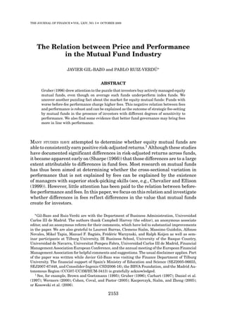
- 9. Price and Performance in the Mutual Fund Industry 2161 of −1.4 and a standard error of 0.34. (Weighting the monthly slope coefficients by the number of observations in each month yields a coefficient of −0.76 with a standard error of 0.23.) Therefore, when we take into account the possibility of correlated residuals in our estimation of standard errors, we also reject, at any conventional significance level, the hypothesis that the slope of the fee- performance relation is one. Moreover, our estimate of the slope coefficient is negative and significantly different from zero at the 5% (1%) significance level when we use clustered (Fama–MacBeth) standard errors to perform our tests. A potential problem with our results is that estimated alphas contain funds’ true abnormal performance, but they also contain estimation error from two sources, the residuals of the performance attribution model (1) and estimation error in the realized risk premium. Estimation error in the dependent vari- able in (2) may affect inference in several ways. First, this estimation error increases the variance of the residuals and thus the standard errors of parame- ter estimates. Therefore, estimation error in alphas decreases the likelihood of finding a significant relationship between alphas and expense ratios. Second, if extreme alphas are more likely to include a large estimation error and have a large inf luence on the estimated coefficient, then estimation error in alphas may affect the estimated slope coefficient. More generally, even in the absence of estimation error in alphas, our results could be driven by a relatively small number of funds with extreme alphas or expenses. To explore the monotonicity and linearity of the fee-performance relation, Figure 1 shows conditional expected risk-adjusted performance as a nonpara- metric function of expenses. We estimate the conditional expectation by us- ing the Nadaraya–Watson estimator with a Gaussian kernel (see, for example, ¨ Hardle (1990)). We also plot conditional expected alphas as a linear function of expenses as implied by the estimated OLS coefficient of the linear regression. To account for time effects, we de-mean expenses and risk-adjusted performance by subtracting the month’s average. For values of expenses below the sample’s 99th percentile, Figure 1 shows that before-expense risk-adjusted performance decreases monotonically with expenses and that the relation may be well de- scribed by a linear function. However, for funds with expenses in the top sample percentile, the relation appears far from monotonic, although the large confi- dence intervals in this low density region suggest that inference on the mean risk-adjusted performance of very expensive funds is problematic. Therefore, Figure 1 shows that the presence of some funds with both extreme expense ratios and extreme risk-adjusted performance does not seem to affect the OLS slope coefficient. Finally, although all funds are affected by estimation error in betas, the stan- dard errors of estimated betas may vary across funds in systematic ways. Thus, although White (1980) and clustered standard errors already account for het- eroskedasticity, we also run several generalized least squares regressions, ob- taining results (see the Internet Appendix) that are essentially identical to those obtained by OLS.
- 10. 2162 The Journal of Finance R 0.04 0.03 0.02 0.01 0 −0.01 −0.02 4-Factor Alpha −0.03 −0.04 −0.05 −0.06 −0.07 −0.08 −0.09 −0.1 −0.11 −0.12 0 0.005 0.01 0.015 0.02 0.025 0.03 0.035 0.04 Expense Ratio 0.05 0.04 4-Factor Alpha (Cross-sectionally Demeaned) 0.03 0.02 0.01 0 −0.01 −0.02 −0.03 −0.04 −0.05 −0.06 −0.07 −0.08 −0.09 −0.1 −0.11 −0.015 −0.01 −0.005 0 0.005 0.01 0.015 0.02 0.025 Expense Ratio (Cross-sectionally Demeaned) Figure 1. Nonparametric Regressions. The figure shows mutual fund conditional expected risk-adjusted performance as a nonparametric function of expense ratios (solid thick line). Risk- adjusted performance in month t is estimated as the difference between the fund’s monthly return in month t and the product of betas and the factor realizations for that month using Carhart’s four-factor model. Both monthly risk-adjusted performance and expense ratios are annualized. The conditional expectation has been estimated using the Nadaraya–Watson estimator with a Gaussian kernel. Dotted lines show upper and lower bounds of the 95% pointwise confidence interval. The figure also plots conditional expected alphas as a linear function of expenses as implied by the estimated OLS coefficient of the linear regression (solid thin line). Dashed vertical lines correspond to the 1st and 99th percentiles of the expense ratio sample distribution. The bottom panel displays the results obtained when we de-mean expenses and risk-adjusted performance by subtracting the month’s sample average.
- 11. Price and Performance in the Mutual Fund Industry 2163 To further account for potential estimation error in alphas stemming from the estimation of betas, we also report results obtained using other performance evaluation models. The last row of Table II shows the results that we obtain when we estimate alpha using the Fama–French three-factor model. The es- timated coefficient is −0.2 with a standard error of 0.26. Therefore, we can reject the null hypothesis that the slope of the fee-performance relation is one at the 1% significance level. However, the estimated coefficient is not signif- icantly different from zero, in contrast to the results obtained with Carhart’s four-factor alpha. This finding suggests that on average, more expensive funds exhibit greater exposure to the momentum factor. Further, in addition to the three- and four-factor unconditional models, we use several conditional versions of Carhart’s four-factor model (see, for example, Ferson and Schadt (1996) and Kosowski et al. (2006)) and obtain results consistent with those from the uncon- ditional model. In the Internet Appendix, we describe in detail the specification and results of the conditional models. Another possible concern about our results is that they may be due to the inf luence of funds with small market share. Such funds may exhibit both low performance and high expense ratios. However, our requirement that funds have at least 48 months of return information to be included in the sample already filters out the effect of unsuccessful funds that are terminated before reaching that threshold. To evaluate the inf luence of small funds that have sur- vived for at least 5 years, we reestimate equation (2) for a sample that excludes observations with relatively low values of assets under management in each month. Panel A of Table III shows that the negative relation between expense ratios and before-expense risk-adjusted performance holds when the lowest size decile is excluded each month. Although the estimated coefficient is signif- icantly different from one at the 1% significance level, it is smaller in absolute value than our estimate for the whole sample and only marginally significantly different from zero. Excluding further deciles leads to similar coefficients and standard errors (with coefficients that are either not statistically significant or only marginally so). Thus, fund size appears to play a role in explaining the relation between risk-adjusted performance and fund expenses. In the analysis above, we consider expense ratios as the only explicit cost of delegated portfolio management. However, investors often pay loads at the time of purchasing and/or redeeming mutual fund shares. Hence, the previous regressions could be capturing a negative relation between performance and a specific component of total fund share ownership cost, but not necessarily a negative relation between performance and the total fees paid by investors. In particular, if more expensive funds (when only expenses are considered) charged lower loads, then after-fee performance (when all fees are considered) could still be equalized across funds. One way to circumvent this problem is to focus exclusively on funds for which annual operating expenses account for 100% of all fees. In Table III (Panel B), we estimate equation (2) for no-load funds only. The estimated slope coefficient of −0.91, which is significant at the 1% level, indicates that total ownership cost and performance are negatively correlated for no-load funds.
- 12. 2164 The Journal of Finance R Table III Regressions by Subsamples The table shows estimated slope coefficients for the OLS regression of funds’ monthly before-fee risk-adjusted performance on monthly fees in the period from January 1962 to December 2005 for Panels A to C, and the period from January 1992 to December 2005 for Panel D. Betas are estimated using Carhart’s four-factor model with a 5-year estimation period. Risk-adjusted performance in month t is the difference between the fund’s monthly before-expense return and the product of betas and the factor realizations in t. Monthly fees are defined as the annual expense ratio divided by 12, except for Panel B, where monthly fees are annual expense ratios divided by 12 plus the sum of front-end and back-end loads divided by the assumed holding period in months. In Panel A the sample does not include for each month the decile of fund-month observations with the lowest total net assets among all actively managed retail funds. In Panel B No-Load Funds are defined as those charging no front- or back-end loads. All regressions include dummies for months. Standard errors (in parentheses) are clustered by time. Adjusted R2 statistics are reported in percentage. ∗ , ∗∗ , ∗∗∗ indicate statistical significance at the 10%, 5%, and 1% levels, respectively. Superscripts a, b, and c denote that the null hypothesis of a unit coefficient is rejected at the 10%, 5%, and 1% significance levels, respectively. Subsample Coefficient Adj. R2 Obs. Panel A: Effect of Small Funds Deciles 2–10 −0.4602∗,c 10.28 225,450 (0.2693) Panel B: Other Fees No-load funds −0.9099∗∗∗,c 8.51 81,323 (0.3220) Load funds (2-year holding period) −0.2660∗∗∗,c 11.22 150,148 (0.1003) Load funds (7-year holding period) −0.5186∗,c 11.22 150,148 (0.2823) Panel C: Regressions by Subperiods 1967–1976 −0.9938b 14.26 16,504 (0.9190) 1977–1986 −0.9581∗,c 8.81 26,591 (0.5625) 1987–1996 −0.8129∗∗∗,c 5.65 39,567 (0.2560) 1997–2005 −0.5384c 10.43 149,724 (0.3347) Panel D: Regressions by Investment Objective Aggressive growth funds −0.4304a 17.44 13,419 (0.7244) Growth MidCap funds −0.0183a 27.99 15,366 (0.6181) Growth and income funds −0.5840∗∗∗,c 12.79 39,221 (0.1619) Growth funds −0.6557∗∗,c 8.48 70,277 (0.2757) Small company growth funds −0.6931∗,c 21.88 35,065 (0.3974)
- 13. Price and Performance in the Mutual Fund Industry 2165 Because load funds constitute two-thirds of the sample, we also estimate the relation between performance and a measure of total fund ownership cost for these funds. Following Sirri and Tufano (1998), we compute total annual owner- ship costs by adding annuitized total loads (total loads divided by the number of years, τ , that investors keep their money in the fund) to annual expense ratios. Although previous studies typically set τ = 7, redemption rates for equity funds for more recent periods suggest a shorter average holding period in the range of 2.5 to 5 years. Therefore, we perform the analysis for τ = 2 and 7 years. Because the analysis in Table III is conducted at a monthly frequency, the independent variable is total monthly ownership cost, defined as total annual ownership cost divided by 12. Panel B of Table III shows that total ownership cost is neg- atively and significantly associated with before-fee risk-adjusted performance for both holding periods. Further, the unit slope hypothesis is rejected at any conventional significance level. As a final test of the robustness of our regression results, we estimate equa- tion (2) for different subperiods and mutual fund categories. Panel C of Table III shows that the perfectly competitive equilibrium condition is clearly violated in all subperiods considered. Moreover, the relation between before-fee risk- adjusted performance and expenses is negative in all the subperiods, although not significantly different from zero in the 1967 to 1976 and 1997 to 2005 sub- periods. Lack of significance in the 1967 to 1976 subperiod could be due to the relatively low number of observations, which results in a large standard error for the slope coefficient. However, failure to reject the null hypothesis of a zero coefficient in the last subperiod appears to happen because the fee-performance relation becomes f latter in the last years of our sample: Although the estimated slope coefficient lies between −0.81 and −0.99 in the pre-1997 years, it is −0.54 in the last subperiod considered. Finally, for the 1992 to 2005 period, for which the classification is detailed and consistent, we divide the sample into subsamples according to the Standard & Poor’s detailed objective code as reported by CRSP, and then run the regres- sion for each subsample. Panel D of Table III shows that expense ratios are negatively related to performance for all five investment objectives, although the relation is not statistically significant for Aggressive Growth and Growth MidCap funds. For these investment objectives, the unit slope hypothesis can be rejected, but only at the 10% significance level. When we replace expense ratios with total ownership cost with τ = 2 or 7 years, we obtain results that are similar to those of Panel D (see the Internet Appendix for results). IV. Explaining the Relation between Fees and Performance The negative relation between before-fee performance and fees that we un- cover in the previous section is at odds with the intuitive expectation that fees should, at least to some extent, ref lect the value that funds create for investors. In this section, we set forth and test different explanations for this apparently anomalous relation.
- 14. 2166 The Journal of Finance R A. Cost-Based Explanations According to the first explanation, fees simply ref lect the costs of operating the fund. If low costs are associated with better before-fee risk-adjusted perfor- mance, then a univariate regression would result in a negative relation between fees and performance. Fund performance could be positively associated with fund costs if higher costs ref lect higher salaries to attract more talented managers or a larger in- vestment in research tools, but there are also arguments for a negative corre- lation between costs and performance. For instance, there might be economies of scale that lower operating costs for larger funds. In addition, larger size may be associated with better performance if a fund’s size ref lects its past perfor- mance, and performance is persistent. Similarly, older funds might benefit from learning economies, which could be passed on to investors in the form of lower fees. If fund longevity is related to good performance, as would be the case if low-performance funds were more likely to close down, we could observe a neg- ative relation between costs and performance. Finally, higher managerial skill may be associated with both better investment decisions and more efficient management of fund operations, which would translate into lower operating costs. B. Strategic Explanations The second explanation views the negative relation between before-fee per- formance and fees as the result of strategic fee-setting by mutual fund manage- ment companies or other service providers to the fund. One such explanation has been proposed and empirically tested for money market mutual funds by Christoffersen and Musto (2002). On the basis of empirical studies on mutual fund f lows (e.g., Sirri and Tufano (1998)) and survey data on mutual fund in- vestors’ behavior (Capon, Fitzimmons, and Prince (1996), Alexander, Jones, and Nigro (1997)), Christoffersen and Musto argue that mutual fund investors differ in their performance sensitivity. They also argue that funds with a worse per- formance history will have a less performance-sensitive clientele because the performance-sensitive investors will have f led those funds following bad perfor- mance. Therefore, funds with a greater proportion of performance-insensitive investors will charge higher fees because for these funds the reduction in after- fee performance caused by an increase in fees will not translate into a large f low of money out of the fund. It follows that funds with bad past performance will find it optimal to charge higher fees. Christoffersen and Musto’s explanation can be tested by using a measure of the performance sensitivity of each fund’s f lows. ´ Gil-Bazo and Ruiz-Verdu (2008) provide a related strategic explanation for the negative relation between before-fee performance and fees. These authors develop an asymmetric information model of the mutual fund market in which mutual funds differ in their expected performance and investors differ in their ´ performance sensitivity. Gil-Bazo and Ruiz-Verdu show that competition for
- 15. Price and Performance in the Mutual Fund Industry 2167 the money of performance-sensitive investors leads to an equilibrium in which funds that expect to earn higher returns (“good” funds) reduce their fees up to the point at which they effectively price funds that expect lower returns (“bad” funds) out of the performance-sensitive segment of the market. Good funds are able to price bad funds out of the market because the revenues of management companies are determined as a fraction of assets under management. Therefore, for any given fee (expressed as a fraction of asset value), good funds, which can be expected to achieve a larger increase in the value of their assets, will earn higher expected revenues. As a result, there is a fee level at which good funds break even in expectation, and low-performance funds incur an expected loss. Unable to compete for performance-sensitive investors, bad funds raise their fees to extract rents from performance-insensitive investors. Gil-Bazo and ´ Ruiz-Verdu’s predictions can also be tested by using a measure of a fund’s risk- adjusted expected performance. A related explanation for our results is that low-performance funds incur higher marketing costs and those costs are passed on to investors in the form of higher fees. If low-performance funds target performance-insensitive investors and these investors purchase mutual fund shares mostly through brokers, then low-performance funds will incur higher marketing costs than funds sold through more direct distribution channels (e.g., from mutual fund supermar- kets or directly from the management company). Bergstresser, Chalmers, and Tufano (2009) provide evidence that supports this hypothesis. These authors report that on average funds sold through the direct or fund supermarket chan- nels perform better and have lower fees than those sold through the broker channel. The marketing costs of low-performance funds could also be higher if intermediaries have to be compensated for the higher effort or potential loss of reputation associated with selling low-performance funds.9 Alternatively, if un- sophisticated investors are more responsive to advertising and low-performance funds target those investors, then low-performance funds will spend more on advertising because the marginal return of their advertising investment will be higher. These strategic marketing explanations imply that underperforming funds will have higher marketing fees, an implication that we can test with our data. ´ Both Gil-Bazo and Ruiz-Verdu’s (2008) explanation and the strategic mar- keting hypothesis assume that fund management companies form expectations about the future performance of the funds they manage, and that they condi- tion their funds’ fees on those expectations. This assumption seems reasonable because management companies are able to observe all publicly available infor- mation about funds’ portfolio choices and returns, they have access to a wealth of data not available to outsiders (such as high-frequency data on portfolio holdings), and they have the skills to analyze all that information. Further, management companies themselves may strongly inf luence the performance of their funds because they decide how to allocate scarce resources (staff, re- search analysis, underpriced IPOs) among them (Gaspar, Massa, and Matos 9 We thank an anonymous referee for suggesting this possibility.
- 16. 2168 The Journal of Finance R (2006), Guedj and Papastaikoudi (2005)). However, a limitation of these hy- potheses is that they do not explain why, rather than adjusting fees, manage- ment companies do not try to improve the expected performance of their funds by replacing underperforming managers or changing their investment strate- gies. In particular, funds with low expected performance could be turned into closet indexers, guaranteeing a level of performance close to the benchmark. Addressing these limitations is beyond the scope of this paper, but allowing for managers’ replacement or changes in investment strategies may not sub- stantially change the predictions of the strategic explanations. First, not all companies will be able to hire only the managers with the highest expected performance, and mutual funds with less-than-top managers may be able to survive, at least in the medium run, especially in the presence of unsophisti- cated investors. Second, even if closet indexing guarantees that returns do not fall too much below a fund’s benchmark, closet indexers will still underperform funds that have managers who are able to generate positive alphas. Further, a strategy of closet indexing also entails some less-obvious costs. In particular, sophisticated investors will leave a fund that they identify as a closet indexer be- cause closet indexers are dominated in terms of after-fee returns by index funds. Another potential limitation of the strategic explanations is that although many studies document the existence of a significant pool of unsophisticated investors, it is an open question whether unsophistication can persist in the medium or long run. In particular, cheaper or better-performing funds may want to educate performance-insensitive investors to avoid expensive funds. However, Gabaix and Laibson (2006) show that firms may not have incentives to educate investors to avoid “shrouded” costly attributes (product attributes that are hidden by firms, even though they could be almost costlessly revealed). Even though most of Gabaix and Laibson’s analysis focuses on add-ons (product attributes that the consumer can substitute away at a cost), the authors also discuss factors that might limit firms’ incentives to educate unsophisticated investors about unavoidable shrouded costs. C. Fund Governance The strategic explanations discussed earlier implicitly assume that mutual fund fees are set by management companies so as to maximize fee revenues. However, U.S. mutual funds are legal entities that are independent of the com- panies managing their portfolio. Control over the fund is delegated by fund shareholders to a board of directors (or trustees), which is responsible for con- tracting the management of the fund’s portfolio with a management company. Thus, the management fee is not set unilaterally by the management company; rather, it is negotiated with the board of directors. Similarly, the fund’s direc- tors negotiate the fees paid to other service providers, such as distributors or transfer agents. Boards of directors have the fiduciary duty to ensure that those fees ref lect the value for fund investors of the services they are paying for. Despite legal provisions imposing rigorous governance requirements on mu- tual funds, there remain important conf licts of interest that may interfere with
- 17. Price and Performance in the Mutual Fund Industry 2169 fund directors’ fiduciary duty. For instance, management companies select the members of a fund’s initial board of directors. In practice, contract renegotia- tions and changes in the fund’s management company are infrequent (Kuhnen (2005), Warner and Wu (2006)), suggesting that directors’ interests may be more aligned with those of management companies than with those of fund investors. Prior research is not fully conclusive as to whether certain mutual fund gov- ernance structures are able to mitigate these conf licts of interest and lead to lower fees. Although Tufano and Sevick (1997) provide evidence for 1992 that funds with smaller boards and funds with boards that have a higher fraction of independent directors have lower fees, more recent studies (Meschke (2007), Ferris and Yan (2007)) obtain mixed results. We hypothesize that the boards of better-governed funds will approve “fair” or “reasonable” fees in fulfillment of their fiduciary duty. This does not necessarily mean lower fees (although better governance could also result in lower fees), but rather that fees are more in line with the fund’s performance. Therefore, the relation between fees and performance should be positive, or at least f latter, for better-governed funds. Similarly, boards of higher quality may resist more strongly any attempts by management companies and other service providers to charge higher fees in funds with more performance-inelastic investors. If this were the case, the relation between fund fees and performance sensitivity would be f latter for better-governed funds. Although with limitations imposed by the nature of our data, we test these hypotheses using Morningstar’s board quality grade as a measure of fund governance. D. Empirical Strategy To test the empirical validity of the proposed explanations for the negative relation between fees and before-fee risk-adjusted performance, we investigate how fees vary with fund characteristics, f low-to-performance sensitivity, and performance. We assume that fund i’s fee at time t, fit , is a linear function of a vector xit−1 of lagged values of variables that are likely to determine the fund’s operating costs, the performance-sensitivity of the fund’s f lows, Sit , and the fund’s expected before-fee performance in period t, αit : f it = γ xit−1 + λ S Sit + λα αit + νit , (3) where νit is a generic error term. Because data on most variables are available yearly during most of the sample period, the time index t in equation (3) refers to calendar years. To test the potential effects of fund governance on fund fees, we also esti- mate an extended version of equation (3) that allows both the intercept and the coefficients on performance and performance sensitivity to depend on board quality. We build on the literature on mutual fund fee determinants, which mostly considers fund fees as a ref lection of operating costs, to select the variables that
- 18. 2170 The Journal of Finance R may inf luence the costs of operating a fund.10 For every fund-year observation we consider the following variables: size, which we define as the log of the year- end total net asset value; age, computed as the log of the number of years since the fund’s organization; size of the complex and number of funds in the complex, which we define as the log of the total net asset value of the funds managed by the company that manages the fund, and the total number of funds managed by that company, respectively; reported annual turnover; volatility, computed as the standard deviation of the fund’s monthly returns in the year; and dummy variables for the fund’s investment objective. We also include a dummy variable to identify single-class load funds and dummies for the main share classes. Doing so makes it possible for us to correct for the potential distortions induced by using a homogeneous holding period for all funds because we can expect investors with different holding periods to select different share classes. We include time dummies in all regressions. We use αit , which we define as the sum of estimated monthly alphas in year t, as our proxy for the fund’s expected before-fee performance.11 Estimated alpha (αit ) is a good measure of expected performance (αit ) as long as the measure- ment error in αit is not correlated with the level of fees. If no such correlation exists, the result of including estimated, rather than expected, performance as a regressor reduces to the well-known attenuation bias in the presence of measurement error. Thus, the performance coefficient estimates are likely to be biased toward zero. To obtain a measure of the f low-to-performance sensitivity, Sit , we proceed in two steps. First, we estimate a model of money f lows into mutual funds. Based on prior studies of fund f low determinants, we allow the sensitivity of f lows to past performance to depend on both the level of performance and fund characteristics. In the second step, we estimate f low-to-performance sensitivity for each fund and year as the first derivative of conditional expected f low with respect to the previous year’s performance. The Appendix provides a detailed description of the construction of this variable. E. The Determinants of Fund Fees To investigate the relation between before-fee performance and the total fees paid by investors, we first use total ownership cost as our dependent vari- able. We compute total ownership cost as the expense ratio plus total loads di- vided by seven. Since we consider a 7-year holding period, to account for usual 10 Different aspects of mutual fund fee determination have been studied, among others, by Fer- ris and Chance (1987), Tufano and Sevick (1997), Latzko (1999), Malhotra and McLeod (1997), Chalmers, Edelen, and Kadlec (2001), Luo (2002), Deli (2002), and Golec (2003). 11 In the remainder of the paper, we focus on unconditional Carhart’s alpha exclusively. We use αit as a measure of the alpha expected by the manager of fund i at the beginning of period t under the assumption that fees are set at the beginning of period t. If fees were set in the middle of period t, our measure of expected performance would thus aggregate performance observed prior to setting fees with expected performance. We have estimated the fee equation using αit+1 as a measure of expected returns and obtained identical results.
- 19. Price and Performance in the Mutual Fund Industry 2171 Table IV Mutual Fund Fee Determinants The table reports estimated coefficients for yearly regressions of funds’ fees on selected fund char- acteristics in the 1993 to 2005 period. The dependent variable in columns (1) to (6) is total annual ownership cost (TOC), computed as total loads divided by seven plus the annual expense ratio. In columns (7) and (8), the dependent variable is marketing fees (Mark.), defined as total loads divided by seven plus 12b-1 fees, and nonmarketing fees (N-Mark.), computed as the expense ratio minus 12b-1 fees, respectively. Back-end loads are assumed to be zero for share classes B and C. The coefficients in columns (1) to (3) and (7) to (8) are estimated by pooled OLS. Column (4) reports estimated coefficients for a regression with management company fixed effects. In column (5) all variables are asset-weighted averages at the management company level. Column (6) reports es- timated coefficients for a regression with fund fixed effects. The size of the management company and the number of funds in the management company are denoted by Co. Size and # funds, respec- tively. σt is the standard deviation of the fund’s monthly returns in year t. St denotes the slope of the estimated f low-to-performance relation. αt is the year t four-factor alpha. All regressions include year dummies and dummy variables for the different investment objectives and share classes. All fees are expressed in bp. The table also reports robust standard errors (in parentheses), which are clustered by fund in columns (1) to (3) and (6) to (8), and by management company in columns (4) to (5). The total number of observations and the adjusted R2 of the regression (in percentage) are reported at the bottom of the table. ∗ , ∗∗ , ∗∗∗ indicate statistical significance at the 10%, 5%, and 1% levels, respectively. TOC Mark. N-Mark. (1) (2) (3) (4) (5) (6) (7) (8) Sizet−1 −9.38∗∗∗ −9.77∗∗∗ −9.76∗∗∗ −7.04∗∗∗ −7.25∗∗∗ −6.35∗∗∗ −3.40∗∗∗ (0.70) (0.82) (0.82) (1.02) (0.80) (0.60) (0.54) Aget−1 −4.96∗∗∗ −8.65∗∗∗ −8.63∗∗∗ −12.05∗∗∗ −0.18 −9.91∗∗∗ −2.99∗∗∗ −5.61∗∗∗ (1.55) (1.73) (1.73) (1.69) (0.19) (0.00) (1.10) (1.29) Co. Sizet−1 −1.06 −1.17 −1.14 −3.75∗∗ −12.82∗∗∗ −1.39∗ 7.46∗∗∗ −8.64∗∗∗ (0.73) (0.81) (0.80) (1.75) (1.58) (0.84) (0.64) (0.55) #fundst−1 −0.09 −0.14 −0.14 0.16 1.44∗∗∗ −0.05 −0.66∗∗∗ 0.52∗∗∗ (0.09) (0.10) (0.10) (0.19) (0.53) (0.10) (0.09) (0.06) Turnovert−1 3.29∗∗∗ 3.27∗∗∗ 3.19∗∗∗ 0.14 9.84∗∗∗ 1.93∗∗∗ −0.70 3.92∗∗∗ (0.73) (0.86) (0.86) (1.04) (2.34) (0.82) (0.70) (0.60) σ t−1 42.53∗∗∗ 34.70∗∗∗ 28.18∗∗ 13.09∗ 58.53∗∗ −12.22∗∗∗ 17.89∗∗ 16.33∗∗ (10.45) (11.49) (11.34) (7.62) (27.78) (6.01) (8.73) (7.92) αt −14.65∗∗∗ −18.56∗∗∗ −19.48∗∗∗ −11.74∗∗ −39.16∗∗ −5.10∗ −11.79∗∗∗ −6.94∗ (5.33) (5.64) (5.68) (5.00) (17.77) (2.92) (4.41) (3.67) αt 2 75.84∗∗∗ (27.38) St −7.06∗∗∗ −7.01∗∗∗ −3.81∗∗∗ −6.54∗∗∗ −0.70 −1.18∗ −5.87∗∗∗ (1.11) (1.11) (0.96) (2.10) (0.55) (0.70) (0.82) Obs. 12,709 10,290 10,290 10,290 1,580 10,290 10,284 10,353 Adj. R2 52.11 55.19 55.23 74.67 54.83 94.22 59.17 42.69 practices we assume that effective back-end loads are zero for classes B and C shares. Column (1) in Table IV presents the results of estimating equation (3) without the performance-sensitivity measure. If the negative relation between expected performance and fees were the consequence of the omission of variables (for
- 20. 2172 The Journal of Finance R example, size, age, or turnover) that are likely to determine operating costs and are related to performance, then we would expect the coefficient on expected performance to change sign, or at least to become statistically insignificant once we include these variables in the regression. As column (1) shows, this is not the case: The coefficient on expected performance remains negative and sig- nificantly different from zero. Therefore, cost-based arguments cannot explain why fees and performance are negatively related. Column (2) reports the results of estimating the full model (3), in which we include both performance and performance-sensitivity as regressors. The neg- ative (and statistically significant at the 1% level) coefficient on performance sensitivity suggests that equity mutual funds strategically exploit a low elastic- ity of demand with respect to net performance to increase their fees. Therefore, our results extend the findings of Christoffersen and Musto (2002), which were obtained for a cross-section of money market mutual funds, to the market for actively managed equity mutual funds, for a much larger sample, and with a more precise measure of performance sensitivity. However, the inclusion of performance sensitivity does not eliminate the negative association between expected before-fee risk-adjusted performance and fees. On the contrary, the estimated coefficient in column (2) is not only negative and statistically signif- icant, but higher (in absolute value) than the estimated coefficient in column (1). Thus, elasticity of demand appears to be an important determinant of fees, but does not in itself explain why underperforming funds set higher fees. To clarify the economic significance of these results, the estimated coefficients in column (2) imply that a one-standard deviation increase in annual before-fee risk-adjusted performance is associated with a decrease of 1.38 basis points in annual total ownership cost, while a one-standard deviation increase in perfor- mance sensitivity is associated with a 4.22-basis point decrease in fees per year. To put these figures in perspective, increases of one-standard deviation in fund volatility and turnover are associated with increases in total ownership cost of 1.99 and 4.79 basis points, respectively, while an increase of one standard deviation in fund size is associated with a reduction in total ownership cost of 23.21 basis points. To account for possible nonlinearities, in column (3) we include alpha squared in the regression. The associated positive coefficient suggests that the relation between alpha and fees becomes f latter for funds with higher alphas, although it remains negative for plausible values of alpha. These results indicate that worse-performing funds and those whose in- vestors have a lower performance sensitivity charge higher fees. Because man- agement companies typically manage many funds, the results could be due to differences between management companies, differences within management companies, or a combination of both. Column (4) of Table IV reports the results when we estimate equation (3) including a management company fixed effect to capture time-invariant differences between management companies. The es- timated coefficients indicate that differences in fees within management com- panies are negatively related to differences in alpha or performance sensitiv- ity. Thus, the results are consistent with management companies strategically setting the fees of their different funds to match the funds’ expected
- 21. Price and Performance in the Mutual Fund Industry 2173 performance or the performance sensitivity of their investors.12 The large in- crease in the adjusted R2 of the regression with respect to the R2 obtained in columns (1) to (3) also suggests that there are management company charac- teristics beyond the company’s total size and number of funds that are related to fees. (The joint hypothesis that all management company fixed effects are zero can be rejected at any reasonable significance level.) We also generate ob- servations at the level of the management company by taking asset-weighted averages of all variables, except for complex size and the number of funds in the complex, for which we retain the management company totals. Column (5) of Table IV reports the results of estimating equation (3) at the management company level. For each management company we compute the asset-weighted average of each variable and exclude management companies for which total net assets of funds with information on the variable are less than 75% of the total net assets of the management company. We also exclude management companies with more than one-third of assets under management in index or institutional funds or more than 10% of assets in funds categorized as outliers. The estimated coefficients for alpha and sensitivity indicate that the results obtained at the fund level extend to the management company level. To evaluate whether marketing or nonmarketing fees are responsible for the negative relation between total fees and performance, we reestimate equation (3), replacing the dependent variable with marketing and nonmarketing fees, alternatively. We define marketing fees as the sum of front- and back-end loads divided by seven (except for B and C share classes, for which we only add front- end loads) and 12b-1 fees. We define nonmarketing fees as the expense ratio minus 12b-1 fees. Columns (7) and (8) of Table IV show that both marketing and nonmarketing fees are negatively related to f low-performance sensitivity and to risk-adjusted performance.13 Therefore, the results are consistent with the three strategic explanations discussed in Section IV.B. In particular, the results obtained for marketing fees suggest that marketing variables, such as distribu- tion channel or advertising expenditures, play a significant role in determining mutual fund fees and contribute to explaining the negative fee-performance relation. Although our results are consistent with the strategic fee-setting hypothe- ses, the negative relation between before-fee performance and fees could also be caused by unobserved fund characteristics that have correlations of oppo- site signs with fees and before-fee risk-adjusted performance. To control for time-invariant unobserved heterogeneity and to shed some light on the deter- minants of fee changes, we also estimate the fee equation (3) with fund fixed 12 Our estimates with management company fixed effects might also pick up longitudinal vari- ation at the management company level. To isolate the cross-sectional variation, we also estimate yearly cross-sectional regressions with management company fixed effects and obtain coefficient estimates and standard errors (see the Internet Appendix) for the whole sample period, using the Fama–MacBeth procedure. The resulting coefficients for alpha and performance sensitivity are neg- ative, statistically significant, and only slightly smaller (in absolute value) than the corresponding coefficients obtained without management company fixed effects. 13 Given the large incidence of funds with zero marketing fees, we also estimate a Tobit model and obtain very similar coefficients and standard errors (results available in the Internet Appendix).
- 22. 2174 The Journal of Finance R effects. Column (6) of Table IV shows that the signs of the coefficients on perfor- mance and performance sensitivity remain negative in the fixed effects specifi- cation. Thus, funds appear to alter their fees over time in response to changes in performance in the same direction found in the absence of fund fixed ef- fects.14 However, the coefficients on performance and performance sensitivity are smaller in absolute value than those in column (2) and the latter coefficient is not statistically different from zero at conventional significance levels. The smaller value and reduced statistical significance of the estimated coefficients on performance and performance sensitivity in the fund fixed effects specifi- cation could be due to fees being largely a matter of long-term strategy, or to the existence of adjustment costs that create substantial inertia in fees. The differences between the specifications could also be due to the fact that our performance and performance sensitivity measures are estimated variables that are likely to contain substantial measurement error. This measurement error may have a larger impact on coefficient estimates when we use only time- series variation to estimate them. For example, in the extreme case in which fund managers’ skills are constant over time, the entire time-series variation in alphas would be due to estimation error. At the same time, the cross-sectional variation in estimated performance would allow us to pick up at least part of the effect of the true alpha. We note that there is a possible alternative explanation for the negative rela- tion between fees and before-fee performance that we do not explicitly consider in our analysis. Higher fees could be paying for better tax management or other fund services, such as check writing, web or telephone services, or better shareholder statements, that compensate investors for differences in after-fee performance. Although our data do not enable us to rule out this explanation, there are reasons to believe that its ability to explain our findings is limited. First, the explanation is valid only if the value of these services is negatively re- lated to fund performance. Moreover, if better fund services or more efficient tax management fully compensated investors for lower after-fee performance, then there would be no reason to expect investors’ money to f low into funds with higher after-fee performance. The explanation also finds little support from the empirical evidence on both the perceived and actual value of fund services, which seem to be limited (Capon, Fitzimmons, and Prince (1996), Elton, Gruber, and Busse (2004), Christoffersen, Evans, and Musto (2005), Bergstresser, Chalmers, and Tufano (2009)). The fact that we find a negative relation be- tween fees and performance when we include fund fixed effects also casts doubt on the plausibility of this interpretation, unless the level of services changes over time in a direction opposite to performance. F. Fund Governance and Fees To analyze the role played by fund governance in the determination of fees, we create dummy variables corresponding to each one of the Morningstar board 14 In tests available in the Internet Appendix, we also estimate the fee equation in differences, as well as logit and probit regressions for the probability of fee changes, and obtain similar results.
- 23. Price and Performance in the Mutual Fund Industry 2175 quality grades. Because only one fund in our sample received Morningstar’s lowest board quality rating, we create a single dummy for the Very Poor and Poor categories, which we refer to as “Poor.” We also create interaction variables of board-quality dummies with before-fee risk-adjusted performance and with our f low-to-performance sensitivity measure. In Table V, we present our regression results. Because of the limitations of our governance subsample, discussed in Section I, these results should be interpreted with caution. First, the fact that our governance information cor- responds to the end of the sample period makes a causal interpretation of the governance coefficients problematic and implies that the results may be sub- ject to survivorship bias. Further, the governance subsample is not a random sample of the population. As we describe in Section I, funds in the governance subsample tend to have lower-than-average fees and higher-than-average per- formance. Keeping these caveats in mind, the results in columns (1) to (5) of Table V provide some support for the hypothesis that better board quality leads to fees that better ref lect the value generated by mutual funds, and that better board quality also limits the ability of management companies to extract rents from performance-insensitive investors. Column (1) presents the results of estimating the fee equation when we ex- clude the performance and performance sensitivity terms, but allow the inter- cept to depend on the board quality grade. In the table, we omit the dummy variable for the Poor grade, so coefficients associated with Fair, Good, or Ex- cellent grades represent differences with respect to funds with a Poor grade. Funds with Good and Excellent grades are associated with lower total own- ership costs than Poor and Fair funds, although the difference between the coefficients associated with Excellent and Poor grades is not statistically dif- ferent from zero. Column (2), which reports the results of estimating the full model, also implies that for most values of before-fee alpha or performance sen- sitivity in the sample, funds with Good or Excellent grades are predicted to be cheaper, all other things equal, than funds with Poor or Fair grades (although this conclusion cannot be directly inferred from the table because the difference between the fees of two funds identical in every respect except for their board quality grade is not just captured by the intercept, but depends on the levels of alpha and performance sensitivity). Thus, columns (1) and (2) suggest that better board quality is associated with lower total ownership costs. However, although in no case are the total ownership costs of a fund with a higher board quality grade significantly higher than those of a fund with a lower grade, some of the estimated differences are not statistically significant and the levels of the estimated coefficients are not strictly monotonic in board quality. If better board quality brings fees more in line with performance, then the coefficient on before-fee performance should be negative for poorly governed funds and the interaction coefficients should be positive and increasing in board quality. The estimated coefficients on performance in column (2) are consistent with this hypothesis. The coefficients on performance sensitivity point in the same direction, but in this case none of the differences is statistically significant at conventional significance levels.
- 24. 2176 The Journal of Finance R Table V Fund Governance and Fees The table reports estimated coefficients for the pooled OLS regression of funds’ fees on selected fund characteristics in the 1993 to 2005 period, except for columns (6) and (7), where the sample period is 2003 to 2005. In columns (1) and (2) the dependent variable is fund total annual ownership cost (TOC), computed as total loads divided by seven plus the annual expense ratio. In column (3) the dependent variable is the asset-weighted average at the management company level of total annual ownership costs. All regressors in column (3) are also asset-weighted averages at the management company level of the corresponding fund-level variables, except for the size of the management company (Co. Size) and the number of funds in the management company (# funds), which are management company totals. In column (4) the dependent variable is marketing fees (Mark.), defined as total loads divided by seven plus 12b-1 fees. Back-end loads are assumed to be zero for share classes B and C. In columns (5) and (7) the dependent variable is nonmarketing fees (N-Mark.), computed as the expense ratio minus 12b-1 fees. Column (6) shows results for management fees (Mgmt.). σt is the standard deviation of the fund’s monthly returns in year t. αt is year t’s four-factor alpha. St denotes the slope of the estimated f low-to-performance relation. Fair, Good, and Excell. are dummy variables that take a value of one if the observation has Fair, Good, or Excellent board quality grade, respectively, and zero otherwise. All regressions include year dummies and dummy variables for the different investment objectives and share classes. All fees are expressed in bp. The table also reports robust standard errors (in parentheses) clustered by fund in all columns except column (3), in which they are clustered by management company. The total number of observations and the adjusted R2 of the regression (in percentage) are reported at the bottom of each column. ∗ , ∗∗ , ∗∗∗ indicate statistical significance at the 10%, 5%, and 1% levels, respectively. Mgmt. N-Mark. TOC TOC TOC Mark. N-Mark. (2003–2005) (2003–2005) (1) (2) (3) (4) (5) (6) (7) Sizet−1 −6.87∗∗∗ −7.93∗∗∗ −6.14∗∗∗ −1.83∗∗∗ −0.46 −1.85∗∗∗ (0.61) (0.98) (0.97) (0.55) (0.44) (0.53) Aget−1 −2.98∗∗∗ −10.50∗∗∗ −0.53∗∗ −1.43 −9.07∗∗∗ −6.01∗∗∗ −7.21∗∗∗ (1.01) (1.69) (0.26) (1.64) (1.21) (1.19) (1.41) Co. Sizet−1 −1.16 0.53 −3.25∗ 7.87∗∗∗ −7.33∗∗∗ −4.40∗∗∗ −8.37∗∗∗ (0.77) (1.05) (1.72) (0.95) (0.63) (0.72) (0.82) # fundst−1 −0.16∗ −0.37∗∗∗ −0.20 −0.71∗∗∗ 0.34∗∗∗ −0.02 0.44∗∗∗ (0.09) (0.12) (0.33) (0.12) (0.07) (0.07) (0.08) Turnovert−1 −0.58 −2.64∗ −2.05 −5.21∗∗∗ 2.58∗∗ 1.09 1.29 (1.12) (1.48) (4.19) (1.52) (1.06) (1.03) (1.25) σ t−1 −5.51 3.82 41.91 −5.52 9.25 29.99∗ 38.60∗∗ (10.95) (16.12) (35.98) (15.77) (10.46) (17.11) (17.45) Fair 4.77 5.03 −2.33 19.75∗∗∗ −14.69∗∗∗ −12.98∗∗∗ −17.06∗∗∗ (4.50) (5.81) (21.28) (4.52) (4.39) (3.06) (4.38) Good −9.83∗∗ −17.12∗∗∗ −19.03 −1.94 −15.05∗∗∗ −9.40∗∗∗ −19.06∗∗∗ (4.40) (5.93) (19.17) (4.73) (4.19) (3.17) (4.22) Excell. −7.95 −13.74∗ −38.63∗ 5.72 −19.33∗∗∗ −10.69∗∗∗ −19.52∗∗∗ (5.11) (7.09) (21.36) (5.88) (4.88) (3.76) (5.00) αt ˆ −50.70∗∗ −104.83 −2.06 −48.57∗∗∗ 9.12 −17.50 (22.70) (116.06) (15.41) (15.08) (24.14) (40.89) αt Fair ˆ 28.15 35.53 −42.82∗∗ 71.05∗∗∗ −3.01 67.03 (24.52) (116.67) (18.42) (16.81) (27.19) (44.59) αt Good ˆ 57.35∗∗ 157.18 1.90 54.74∗∗∗ 2.62 61.96 (24.27) (114.03) (17.24) (15.72) (28.92) (43.64) (continued)
- 25. Price and Performance in the Mutual Fund Industry 2177 Table V—Continued Mgmt. N-Mark. TOC TOC TOC Mark. N-Mark. (2003–2005) (2003–2005) (1) (2) (3) (4) (5) (6) (7) αt Excell. ˆ 61.63∗∗ 106.99 19.90 41.32∗∗ −72.74∗∗ −41.67 (26.42) (112.55) (18.60) (17.54) (35.48) (51.16) St −8.59 −7.71 6.01∗ −14.91∗∗∗ −6.08 −17.22∗∗∗ (5.37) (18.35) (3.52) (4.08) (3.98) (4.37) St Fair 3.60 −12.43 −9.15∗∗ 12.99∗∗∗ 6.14 17.52∗∗∗ (5.94) (19.30) (4.37) (4.36) (4.19) (4.69) St Good 7.31 6.28 −3.09 10.56∗∗ 4.11 12.90∗∗∗ (5.70) (18.05) (4.00) (4.23) (4.33) (4.58) St Excell. 4.97 15.06 −12.21∗∗ 17.14∗∗∗ 10.31∗ 16.08∗∗∗ (6.50) (19.28) (4.81) (4.93) (5.43) (5.74) Obs. 7,767 3,933 545 3,933 3,971 1,734 1,734 Adj. R2 58.58 67.39 68.64 65.73 46.59 39.51 39.40 Because as mentioned earlier, funds managed by the same management com- pany frequently share the same board, we also reestimate the fee regression at the management company level by taking asset-weighted averages of the variables. Column (3) in Table V reports that the signs of the coefficients of interest are the same as in the previous column, although no coefficient (other than the intercept for funds with an Excellent grade) is significantly different from zero (a result that is not due to a reduced magnitude of the coefficients but to much larger standard errors). Tufano and Sevick (1997) argue that the effect of fund governance should be most visible for management fees, since for these fees we can expect the conf lict of interest between the management company and shareholders to be most severe. However, these authors find little difference in how board char- acteristics are related to marketing and nonmarketing fees. We replicate the analysis carried out in columns (1) and (2) with marketing and nonmarketing fees as dependent variables, although we report only the estimated coefficients of the full model in columns (4) and (5) of Table V, respectively. The results for marketing fees are mixed. Funds with Good and Excellent grades charge lower fees (although in column (4) the intercept for funds with an Excellent grade is marginally higher than that for funds with a Poor grade, the former are cheaper on average, other things equal) and have the highest coefficients on before-fee performance. However, the funds with a Fair grade—not those with a Poor grade—are the ones that charge the highest fees and have the lowest coefficient on before-fee performance. Therefore, there is no monotonicity at the bottom in the relation between board quality and marketing fees. Further, the differences between funds with a Poor grade and funds with a Good or Excel- lent grade are not statistically significant. Finally, the sensitivity coefficients follow no clear pattern: The lowest (and negative) coefficient corresponds to funds with the highest board quality grade. The results for nonmarketing fees are more in line with those in columns (1) and (2). When we estimate the same specification as in column (1) (see the
- 26. 2178 The Journal of Finance R Internet Appendix for the results), we find that other things equal, funds with a Poor grade charge the highest nonmarketing fees, and funds with Good and Excellent grades charge the lowest nonmarketing fees (which is the same or- dering as the one implied by the intercepts in column (5)). The relation between performance sensitivity and nonmarketing fees becomes f latter as board qual- ity improves: The sensitivity coefficient is −14.91 for funds with a Poor grade and the estimated differences imply that the same coefficient for funds with an Excellent grade is 2.23. However, further tests indicate that this coefficient is not significantly different from zero. Finally, funds with a Poor grade have a negative coefficient on performance. This coefficient is significantly lower than the coefficients for all other grades, although the coefficients for the higher grades are not increasing in board quality. Therefore, the results are consistent with the hypothesis that better-governed funds resist attempts by manage- ment companies to exploit investors’ low performance sensitivity. The results also provide weaker evidence for the hypothesis that better board quality brings nonmarketing fees more in line with fund performance. Since CRSP started providing data on management fees as of 2003, we can perform the analysis with management fees as the dependent variable for the 2003 to 2005 period. When we estimate a specification such as the one in col- umn (1), we again find that the worst-governed funds charge the highest fees, as suggested by the ordering of the intercept coefficients reported in column (6). Further, the differences between the sensitivity coefficients are similar to those in column (5), although the statistical significance of the coefficients is marginal at best. However, the performance coefficients follow no clear pattern: The coefficient for the best-governed funds is not only negative but lower than all other coefficients, a result that is in stark contrast with those in columns (1) to (5). To check whether this result is due to a different behavior of manage- ment fees or to the different sample period, we reestimate the equation with nonmarketing fees, which are the closest approximation to actual management fees, as the dependent variable for the 2003 to 2005 period, and report the re- sults in column (7) of Table V. Although the size and statistical significance of the performance coefficients vary, the ordering of these coefficients is the same in columns (6) and (7), showing that the best-governed funds have the lowest performance coefficient in both columns. We cannot explain this result. It may be due to an effort by the best-performing among the best-governed funds to lower their fees to compensate mutual fund investors for the decline in the stock markets during the 2000–2002 period, or to a response by these funds to the series of mutual fund scandals that emerged in 2003 and 2004. However, the short sample period, the noise inherent in our performance measure, and the fact that the only significant differences between the full sample and the 2003 to 2005 period have to do with the coefficients on performance suggest caution when interpreting the differences as indicating a structural change. V. Conclusion In this paper we show that there is a negative relation between funds’ before- fee performance and the fees they charge to investors. Since this evidence is at
- 27. Price and Performance in the Mutual Fund Industry 2179 odds with economic intuition, we subject it to a series of robustness tests, and find that it survives all of them. Next, we propose two explanations for this anomalous result. According to the first explanation, the negative relation is the consequence of factors, which are omitted in univariate regressions, that are both positively correlated with returns and negatively correlated with funds’ operating costs, and thus also with fund fees. According to the second explanation, in contrast, the nega- tive relation is the result of funds that strategically set fees as a function of their past or expected performance. We consider three related rationales for this strategic behavior. The first, proposed by Christoffersen and Musto (2002), argues that funds with worse past performance have a pool of investors that are less sensitive to fund performance. Faced with an inelastic demand for their shares, underperforming funds optimally increase fees. The second expla- ´ nation, proposed by Gil-Bazo and Ruiz-Verdu (2008), argues that funds with lower expected performance optimally set higher fees and target performance- insensitive investors, since these funds anticipate that they will not be able to compete with better-performing funds in the market for sophisticated in- vestors. On the other hand, better-performing funds keep fees low because of competition among them for the money of performance-sensitive investors. The third explanation argues that funds with different expected performance choose different marketing strategies. Funds with low expected performance are mar- keted to performance-insensitive investors and have higher distribution costs, which translate into higher fees. The empirical analysis finds support for all strategic-pricing explanations. Even though funds’ operating costs are important determinants of fees, they do not explain away the negative relation between before-fee performance and fees. When we control for those cost determinants, we find that funds with lower expected before-fee performance and funds with less elastic demands charge higher marketing and nonmarketing fees. Therefore, it appears that mutual fund competition and regulation have not been sufficient to ensure that fees ref lect the value that funds create for investors. However, we find some evidence that better fund governance may be associated with fees that are more in line with performance: Among the best-governed funds, worse performance need not mean higher fees. Appendix: Estimation of Flow-to-Performance Sensitivity We define annual net f low to fund i in year t, Flowit , as the relative growth of the fund’s total net assets (TNA) adjusted for returns net of expenses, Rn :15 it TNAit − TNAit−1 1 + Rit n Flowit = . (A1) TNAit−1 15 Elton, Gruber, and Blake (2001) report a number of errors associated with mutual fund mergers and splits in the CRSP sample. Huang, Wei, and Yan (2007) argue that these errors could lead to extreme values of f lows. We deal with this problem by eliminating the 1% of observations with the lowest and highest f lows in each year.