1. Copyright © Rutgers Writing Program
Contact Barclay Barrios (barclay.barrios@rutgers.edu)
Tutorial – Microsoft Office Excel 2003
Introduction:
Microsoft Excel is the most widespread program for creating spreadsheets on the
market today. Spreadsheets allow you to organize information in rows and tables
(which create cells), with the added bonus of automatic mathematics. Spreadsheets
have been used for many, many years in business to keep track of expenses and
other calculations. Excel will keep track of numbers you place in cells, and if you
define cells to refer to each other, any changes made in one cell will be reflected in
these referring cells. It sounds a bit complicated, but Excel makes it all a breeze.
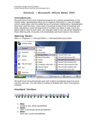
Opening Excel:
Start >> Programs >> Microsoft Office >> Microsoft Office Excel 2003
Microsoft Excel will automatically open with a blank spreadsheet spanning many
columns and rows. You will notice a number of toolbars with many more options
included.
Standard Toolbar:
1. New:
Create a new, blank spreadsheet
2. Open:
Open a previously saved spreadsheet
3. Save:
Save your current spreadsheet
2. Copyright © Rutgers Writing Program
Contact Barclay Barrios (barclay.barrios@rutgers.edu)
4. Permission:
5. Print:
Prints the current document.
6. Print Preview:
Preview the potential print of the current document.
7. Research:
Microsoft has enabled Information Rights Management (IRM) within the new
version of Excel, which can help protect sensitive documents from being
copied or forwarded. Click this for more information and options.
8. Copy:
Copies the current selection to the clipboard, which can then be pasted
elsewhere in the document.
9. Paste:
Takes the current clipboard contents and inserts them.
10. Undo:
Undoes the last action in the document, reverting “back” a step in time.
11. Insert Hyperlink:
Inserts a hyperlink to an Internet location.
12. AutoSum:
A drop-down menu of available mathematical operations to perform.
13. Sort Ascending:
Sorts the current selection in ascending order.
14. Chart Wizard:
Opens the “Chart Wizard,” which will walk you through the creation of a chart
/ diagram using the currently selected information.
15. Microsoft Excel Help:
Brings up the Excel Help window, which will allow you to type in a key-word
for more information, or click anything on screen to directly bring up further
information on that subject.
16. More Options:
There are a variety of extra options you can call or add to the toolbar, such as
Spell Check, Sort Descending, Cut, Redo, etc. By clicking the triangle, you
can access these options; at the same time, you can drag this toolbar
outwards more to make more available space for these options directly on the
toolbar.
Formatting Toolbar:
1. Font:
Change the font of the selected cell(s)
2. Size:
Change the font size of the selection
3. Bold:
Put the selection in bold face
4. Italics:
Italicize the selection
5. Underline:
Underline the selection
3. Copyright © Rutgers Writing Program
Contact Barclay Barrios (barclay.barrios@rutgers.edu)
6. Align Left:
Align the current selection to the left
7. Center:
Align the current selection to the center
8. Align Right:
Align the current selection to the right
9. Merge & Center:
Combine two selected cells into one new cell that spans the width of both and
center the contents of this new cell
10. Currency Style:
Change the style in which currency is displayed
11. Percent Style:
Change the style in which percents are displayed
12. Decrease Indent:
Decrease the indent of a cell by approximately one character
13. Border:
Add or alter the style of borders to format a cell with
14. Fill Color:
Select a color to fill the background of a cell with
15. Font Color:
Select a color to apply to a selection of text
You now have a basic understanding of the toolbars, but still have a huge window of
cells in front of you. What can you do with them? Cells can contain text, numbers, or
formulas (don't worry about formulas quite yet). To refer to a particular cell, you call
it by its column letter, and then by its row letter. For example, the cell in the
uppermost left corner would be "A1." The current cell(s) will always be listed in the
"Name Box," which appears on the left below the toolbars.
Navigating the Spreadsheet:
You can use the "Up," "Down," "Left," "Right," to move (one cell at a time)
throughout the spreadsheet. You can also simply click the cursor into a cell). The
"tab" button will move one cell to the right. The "Enter" button will confirm the
entered information and move one cell down.
If you enter text or numbers that span further than the column allows, simply place
your cursor on the line dividing two columns next to their respective letters, and
drag to the right or left until the desired width is achieved. You can also double-click
this dividing line to have Excel automatically choose the best width.
4. Copyright © Rutgers Writing Program
Contact Barclay Barrios (barclay.barrios@rutgers.edu)
A Simple Spreadsheet:
This is what a basic spreadsheet may look like, keeping track of the grades for five
students. As you'll notice, numbers automatically align to the right, while text
automatically aligns to the left. Room has been allowed at the top and the left for
column and row headings, which have been placed in bold.
Simple Formulas:
"92.67" was not entered as the contents for cell "E2." The "formula bar" has the
following entered into it:
=(B2+C2+D2)/3
By following the normal order of operations, the contents of the three cells in
parenthesis (B2, C2, and D2) are all added to each other, and then divided by 3. This
gives an average of the three grades, which is then shown in the cell "E2" (where the
formula was entered).
If you wanted to do the same for students 2 through 5, you would enter in similar
formulas for each cell from "E3" to "E6" replacing the column and row numbers
where appropriate.
An easy method to replicate formulas is to select the cell which contains the original
formula ("E2" in this case), click the bottom right corner of the selection box, and
drag down several rows (to "E6" in this example). The formula will be copied down in
each cell, and will change itself to reflect each new row.
5. Copyright © Rutgers Writing Program
Contact Barclay Barrios (barclay.barrios@rutgers.edu)
Insert Rows & Columns:
You may find that you need to insert a new, blank row where there isn't a blank row
any more. To insert a new blank row, place your cursor directly below where you
would like a new row. Select Insert >> Rows. To insert a new column, place the
cursor in a cell directly to the right of where you would like the column. Select Insert
>> Columns.
Sorting:
One of Excel’s powerful features is its ability to sort, while still retaining the
relationships among information. For example, let’s take our student grade example
from above. What if we wanted to sort the grades in descending order? First, let’s
select the information we want to sort.
Now let’s select the “Sort” option from the “Data” menu.
A new window will appear asking how you would like to sort the information. Let’s
sort it by the average grade, which is in Column E; be sure to set by “Descending”
6. Copyright © Rutgers Writing Program
Contact Barclay Barrios (barclay.barrios@rutgers.edu)
order. If there were other criteria you wished to sort by as secondary measures, you
could do so; let’s select “Then by” as “Grade 3” just for the practice of doing so
(“Descending” order, as well).
Excel will sort your information with the specifications you entered. The results
should look something like this:
Cell Formatting:
You may notice that, by default, Excel will leave as many decimal points as possible
within the cell’s width restraints; as you increase the cell’s width, the number of
decimal points increases.
Select “Cells” from the “Format” menu. A new window will appear with a wide
variety of ways in which to customize your spreadsheets.
7. Copyright © Rutgers Writing Program
Contact Barclay Barrios (barclay.barrios@rutgers.edu)
For example, if we wanted to set the percentages fixed to only two decimal points,
you can make this selection under the “Number” category within the “Number” tab.
You can also set the formatting for things such as the date, time, currency, etc.
The “Font” tab will also allow you to change the default font used on the
spreadsheet. The other tabs provide even more ways to customize your spreadsheet
and its appearance; experiment with the settings to see what works best for you.
Chart Wizard:
Excel allows you to create basic – to – intermediate charts based off of information
and data within your spreadsheets. Let’s create a column chart from the student
grade data from before. First, highlight the data.
Next, select “Chart” from the “Insert” menu.
8. Copyright © Rutgers Writing Program
Contact Barclay Barrios (barclay.barrios@rutgers.edu)
A new window will appear asking which type of chart you would like to create. For
this example, let’s do a basic pie chart. Select “Column” from the “Chart Type” on
the left side, and pick the first sub-type on the right (a normal, 2D column chart).
Click “Next.” In this window, you’ll be asked to select your “data range”; this is the
area of your spreadsheet that you wish to generate a chart from. Since you’ve
already selected the area before, it should already be entered into the appropriate
area. “Series in” allows you to choose by which value you want to arrange the chart.
Let’s arrange it by rows; this will break it down by “Grade” (such as Test 1, Test 2,
etc.) and comparing the student scores next to each other.
9. Copyright © Rutgers Writing Program
Contact Barclay Barrios (barclay.barrios@rutgers.edu)
Click “Next.” In step three you can give the chart a name (“Chart Title”), label the X
and/or Y axis, etc.
10. Copyright © Rutgers Writing Program
Contact Barclay Barrios (barclay.barrios@rutgers.edu)
Click “Next.” The final step will ask whether you want the chart as an object in your
current spreadsheet or in a new one; generally, you will place it within the same
spreadsheet.
Click “Finish,” and your chart will appear in your spreadsheet!