1. TOPIC MODELS
DAVID M. BLEI
PRINCETON UNIVERSITY
JOHN D. LAFFERTY
CARNEGIE MELLON UNIVERSITY
1. I NTRODUCTION
Scientists need new tools to explore and browse large collections of schol-
arly literature. Thanks to organizations such as JSTOR, which scan and
index the original bound archives of many journals, modern scientists can
search digital libraries spanning hundreds of years. A scientist, suddenly
faced with access to millions of articles in her field, is not satisfied with
simple search. Effectively using such collections requires interacting with
them in a more structured way: finding articles similar to those of interest,
and exploring the collection through the underlying topics that run through
it.
The central problem is that this structure—the index of ideas contained
in the articles and which other articles are about the same kinds of ideas—is
not readily available in most modern collections, and the size and growth
rate of these collections preclude us from building it by hand. To develop
the necessary tools for exploring and browsing modern digital libraries, we
require automated methods of organizing, managing, and delivering their
contents.
In this chapter, we describe topic models, probabilistic models for uncov-
ering the underlying semantic structure of a document collection based on a
hierarchical Bayesian analysis of the original texts Blei et al. (2003); Grif-
fiths and Steyvers (2004); Buntine and Jakulin (2004); Hofmann (1999);
Deerwester et al. (1990). Topic models have been applied to many kinds
of documents, including email ?, scientific abstracts Griffiths and Steyvers
(2004); Blei et al. (2003), and newspaper archives Wei and Croft (2006).
By discovering patterns of word use and connecting documents that exhibit
similar patterns, topic models have emerged as a powerful new technique
for finding useful structure in an otherwise unstructured collection.
With the statistical tools that we describe below, we can automatically or-
ganize electronic archives to facilitate efficient browsing and exploring. As
a running example, we will analyze JSTOR’s archive of the journal Science.
1

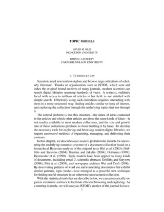
2. 2 D. M. BLEI AND J. D. LAFFERTY
computer chemistry cortex orbit infection
methods synthesis stimulus dust immune
number oxidation fig jupiter aids
two reaction vision line infected
principle product neuron system viral
design organic recordings solar cells
access conditions visual gas vaccine
processing cluster stimuli atmospheric antibodies
advantage molecule recorded mars hiv
important studies motor field parasite
F IGURE 1. Five topics from a 50-topic LDA model fit to
Science from 1980–2002.
Figure 1 illustrates five “topics” (i.e., highly probable words) that were dis-
covered automatically from this collection using the simplest topic model,
latent Dirichlet allocation (LDA) (Blei et al., 2003) (see Section 2). Further
embellishing LDA allows us to discover connected topics (Figure 7) and
trends within topics (Figure 9). We emphasize that these algorithms have no
prior notion of the existence of the illustrated themes, such as neuroscience
or genetics. The themes are automatically discovered from analyzing the
original texts
This chapter is organized as follows. In Section 2 we discuss the LDA
model and illustrate how to use its posterior distribution as an exploratory
tool for large corpora. In Section 3, we describe how to effectively ap-
proximate that posterior with mean field variational methods. In Section 4,
we relax two of the implicit assumptions that LDA makes to find maps of
related topics and model topics changing through time. Again, we illus-
trate how these extensions facilitate understanding and exploring the latent
structure of modern corpora.
2. L ATENT D IRICHLET ALLOCATION
In this section we describe latent Dirichlet allocation (LDA), which has
served as a springboard for many other topic models. LDA is based on
seminal work in latent semantic indexing (LSI) (Deerwester et al., 1990)
and probabilistic LSI (Hofmann, 1999). The relationship between these
techniques is clearly described in Steyvers and Griffiths (2006). Here, we
develop LDA from the principles of generative probabilistic models.
2.1. Statistical assumptions. The idea behind LDA is to model documents
as arising from multiple topics, where a topic is defined to be a distribution
over a fixed vocabulary of terms. Specifically, we assume that K topics are

3. TOPIC MODELS 3
associated with a collection, and that each document exhibits these topics
with different proportions. This is often a natural assumption to make be-
cause documents in a corpus tend to be heterogeneous, combining a subset
of main ideas or themes that permeate the collection as a whole.
JSTOR’s archive of Science, for example, exhibits a variety of fields, but
each document might combine them in novel ways. One document might
be about genetics and neuroscience; another might be about genetics and
technology; a third might be about neuroscience and technology. A model
that limits each document to a single topic cannot capture the essence of
neuroscience in the same way as one which addresses that topics are only
expressed in part in each document. The challenge is that these topics are
not known in advance; our goal is to learn them from the data.
More formally, LDA casts this intuition into a hidden variable model of
documents. Hidden variable models are structured distributions in which
observed data interact with hidden random variables. With a hidden vari-
able model, the practitioner posits a hidden structure in the observed data,
and then learns that structure using posterior probabilistic inference. Hidden
variable models are prevalent in machine learning; examples include hidden
Markov models (Rabiner, 1989), Kalman filters (Kalman, 1960), phyloge-
netic tree models (Mau et al., 1999), and mixture models (McLachlan and
Peel, 2000).
In LDA, the observed data are the words of each document and the hidden
variables represent the latent topical structure, i.e., the topics themselves
and how each document exhibits them. Given a collection, the posterior
distribution of the hidden variables given the observed documents deter-
mines a hidden topical decomposition of the collection. Applications of
topic modeling use posterior estimates of these hidden variables to perform
tasks such as information retrieval and document browsing.
The interaction between the observed documents and hidden topic struc-
ture is manifest in the probabilistic generative process associated with LDA,
the imaginary random process that is assumed to have produced the ob-
served data. Let K be a specified number of topics, V the size of the vo-
cabulary, α a positive K -vector, and η a scalar. We let DirV (α) denote a
V -dimensional Dirichlet with vector parameter α and Dir K (η) denote a K
dimensional symmetric Dirichlet with scalar parameter η.
(1) For each topic,
(a) Draw a distribution over words βk ∼ DirV (η).
(2) For each document,
(a) Draw a vector of topic proportions θd ∼ Dir(α).
(b) For each word,
(i) Draw a topic assignment Z d,n ∼ Mult(θd ), Z d,n ∈ {1, . . . , K }.

4. 4 D. M. BLEI AND J. D. LAFFERTY
α θd Zd,n Wd,n βk η
N
D K
F IGURE 2. A graphical model representation of the la-
tent Dirichlet allocation (LDA). Nodes denote random vari-
ables; edges denote dependence between random variables.
Shaded nodes denote observed random variables; unshaded
nodes denote hidden random variables. The rectangular
boxes are “plate notation,” which denote replication.
(ii) Draw a word Wd,n ∼ Mult(βz d,n ), Wd,n ∈ {1, . . . , V }.
This is illustrated as a directed graphical model in Figure 2.
The hidden topical structure of a collection is represented in the hidden
random variables: the topics β1:K , the per-document topic proportions θ1:D ,
and the per-word topic assignments z 1:D,1:N . With these variables, LDA
is a type of mixed-membership model (Erosheva et al., 2004). These are
distinguished from classical mixture models (McLachlan and Peel, 2000;
Nigam et al., 2000), where each document is limited to exhibit one topic.
This additional structure is important because, as we have noted, documents
often exhibit multiple topics; LDA can model this heterogeneity while clas-
sical mixtures cannot. Advantages of LDA over classical mixtures has been
quantified by measuring document generalization (Blei et al., 2003).
LDA makes central use of the Dirichlet distribution, the exponential fam-
ily distribution over the simplex of positive vectors that sum to one. The
Dirichlet has density
Γ αi
(1) p(θ | α) = i
θiαi −1 .
i Γ (αi ) i
The parameter α is a positive K -vector, and Γ denotes the Gamma func-
tion, which can be thought of as a real-valued extension of the factorial
function. A symmetric Dirichlet is a Dirichlet where each component of the
parameter is equal to the same value. The Dirichlet is used as a distribu-
tion over discrete distributions; each component in the random vector is the
probability of drawing the item associated with that component.
LDA contains two Dirichlet random variables: the topic proportions θ
are distributions over topic indices {1, . . . , K }; the topics β are distributions
over the vocabulary. In Section 4.2 and Section 4.1, we will examine some

5. TOPIC MODELS 5
contractual employment female markets criminal
expectation industrial men earnings discretion
gain local women investors justice
promises jobs see sec civil
expectations employees sexual research process
breach relations note structure federal
enforcing unfair employer managers see
supra agreement discrimination firm officer
note economic harassment risk parole
perform case gender large inmates
F IGURE 3. Five topics from a 50-topic model fit to the Yale
Law Journal from 1980–2003.
of the properties of the Dirichlet, and replace these modeling choices with
an alternative distribution over the simplex.
2.2. Exploring a corpus with the posterior distribution. LDA provides
a joint distribution over the observed and hidden random variables. The hid-
den topic decomposition of a particular corpus arises from the correspond-
ing posterior distribution of the hidden variables given the D observed doc-
uments w1:D ,
(2) p(θ1:D , z 1:D,1:N , β1:K | w1:D,1:N , α, η) =
p(θ1:D , z 1:D , β1:K | w1:D , α, η)
.
β1:K θ1:D z p(θ1:D , z 1:D , β1:K | w1:D , α, η)
Loosely, this posterior can be thought of the “reversal” of the generative
process described above. Given the observed corpus, the posterior is a dis-
tribution of the hidden variables which generated it.
As discussed in Blei et al. (2003), this distribution is intractable to com-
pute because of the integral in the denominator. Before discussing approxi-
mation methods, however, we illustrate how the posterior distribution gives
a decomposition of the corpus that can be used to better understand and
organize its contents.
The quantities needed for exploring a corpus are the posterior expecta-
tions of the hidden variables. These are the topic probability of a term
βk,v = E[βk,v | w1:D,1:N ], the topic proportions of a document θd,k =
E[θd,k | w1:D,1:N ], and the topic assignment of a word z d,n,k = E[Z d,n =
k | w1:D,1:N ]. Note that each of these quantities is conditioned on the ob-
served corpus.

6. 6 D. M. BLEI AND J. D. LAFFERTY
Visualizing a topic. Exploring a corpus through a topic model typi-
cally begins with visualizing the posterior topics through their per-topic
term probabilities β. The simplest way to visualize a topic is to order the
terms by their probability. However, we prefer the following score,
 
βk,v
term-scorek,v = βk,v log  .
 
(3)  1 
K K
j=1 β j,v
This is inspired by the popular TFIDF term score of vocabulary terms used
in information retrieval Baeza-Yates and Ribeiro-Neto (1999). The first
expression is akin to the term frequency; the second expression is akin to
the document frequency, down-weighting terms that have high probability
under all the topics. Other methods of determining the difference between
a topic and others can be found in (Tang and MacLennan, 2005).
Visualizing a document. We use the posterior topic proportions θd,k
and posterior topic assignments z d,n,k to visualize the underlying topic de-
composition of a document. Plotting the posterior topic proportions gives a
sense of which topics the document is “about.” These vectors can also be
used to group articles that exhibit certain topics with high proportions. Note
that, in contrast to traditional clustering models (Fraley and Raftery, 2002),
articles contain multiple topics and thus can belong to multiple groups. Fi-
nally, examining the most likely topic assigned to each word gives a sense
of how the topics are divided up within the document.
Finding similar documents. We can further use the posterior topic pro-
portions to define a topic-based similarity measure between documents.
These vectors provide a low dimensional simplicial representation of each
document, reducing their representation from the (V − 1)-simplex to the
(K − 1)-simplex. One can use the Hellinger distance between documents
as a similarity measure,
K 2
(4) document-similarityd, f = θd,k − θ f,k .
k=1
To illustrate the above three notions, we examined an approximation to
the posterior distribution derived from the JSTOR archive of Science from
1980–2002. The corpus contains 21,434 documents comprising 16M words
when we use the 10,000 terms chosen by TFIDF (see Section 3.2). The
model was fixed to have 50 topics.
We illustrate the analysis of a single article in Figure 4. The figure depicts
the topic proportions, the top scoring words from the most prevalent topics,

7. TOPIC MODELS 7
Top words from the top topics (by term score) Expected topic proportions
sequence measured residues computer
region average binding methods
pcr range domains number
0.20
identified values helix two
fragments different cys principle
two size regions design
0.10
genes three structure access
three calculated terminus processing
cdna two terminal advantage
low site important
0.00
analysis
Abstract with the most likely topic assignments
Top Ten Similar Documents
Exhaustive Matching of the Entire Protein Sequence Database
How Big Is the Universe of Exons?
Counting and Discounting the Universe of Exons
Detecting Subtle Sequence Signals: A Gibbs Sampling Strategy for Multiple Alignment
Ancient Conserved Regions in New Gene Sequences and the Protein Databases
A Method to Identify Protein Sequences that Fold into a Known Three- Dimensional Structure
Testing the Exon Theory of Genes: The Evidence from Protein Structure
Predicting Coiled Coils from Protein Sequences
Genome Sequence of the Nematode C. elegans: A Platform for Investigating Biology
F IGURE 4. The analysis of a document from Science. Doc-
ument similarity was computed using Eq. (4); topic words
were computed using Eq. (3).
the assignment of words to topics in the abstract of the article, and the top
ten most similar articles.
3. P OSTERIOR INFERENCE FOR LDA
The central computational problem for topic modeling with LDA is ap-
proximating the posterior in Eq. (2). This distribution is the key to using
LDA for both quantitative tasks, such as prediction and document general-
ization, and the qualitative exploratory tasks that we discuss here. Several
approximation techniques have been developed for LDA, including mean
field variational inference (Blei et al., 2003), collapsed variational infer-
ence (Teh et al., 2006), expectation propagation (Minka and Lafferty, 2002),

8. 8 D. M. BLEI AND J. D. LAFFERTY
and Gibbs sampling (Steyvers and Griffiths, 2006). Each has advantages
and disadvantages: choosing an approximate inference algorithm amounts
to trading off speed, complexity, accuracy, and conceptual simplicity. A
thorough comparison of these techniques is not our goal here; we use the
mean field variational approach throughout this chapter.
3.1. Mean field variational inference. The basic idea behind variational
inference is to approximate an intractable posterior distribution over hidden
variables, such as Eq. (2), with a simpler distribution containing free varia-
tional parameters. These parameters are then fit so that the approximation
is close to the true posterior.
The LDA posterior is intractable to compute exactly because the hidden
variables (i.e., the components of the hidden topic structure) are dependent
when conditioned on data. Specifically, this dependence yields difficulty
in computing the denominator in Eq. (2) because one must sum over all
configurations of the interdependent N topic assignment variables z 1:N .
In contrast to the true posterior, the mean field variational distribution for
LDA is one where the variables are independent of each other, with and
each governed by a different variational parameter:
(5)
K D N
q(θ1:D , z 1:D,1:N , β1:K ) = q(βk | λk ) q(θd d | γd ) q(z d,n | φd,n )
k=1 d=1 n=1
Each hidden variable is described by a distribution over its type: the topics
β1:K are each described by a V -Dirichlet distribution λk ; the topic propor-
tions θ1:D are each described by a K -Dirichlet distribution γd ; and the topic
assignment z d,n is described by a K -multinomial distribution φd,n . We em-
phasize that in the variational distribution these variables are independent;
in the true posterior they are coupled through the observed documents.
With the variational distribution in hand, we fit its variational parameters
to minimize the Kullback-Leibler (KL) to the true posterior:
arg min KL(q(θ1:D , z 1:D,1:N , β1:K )|| p(θ1:D , z 1:D,1:N , β1:K | w1:D,1:N ))
γ1:D ,λ1:K ,φ1:D,1:N
The objective cannot be computed exactly, but it can be computed up to a
constant that does not depend on the variational parameters. (In fact, this
constant is the log likelihood of the data under the model.)

9. TOPIC MODELS 9
Specifically, the objective function is
(6)
K D D N
L= E[log p(βk | η)] + E[log p(θd | α)] + E[log p(Z d,n | θd )]
k=1 d=1 d=1 n=1
D N
+ E[log p(wd,n | Z d,n , β1:K )] + H(q),
d=1 n=1
where H denotes the entropy and all expectations are taken with respect to
the variational distribution in Eq. (5). See Blei et al. (2003) for details on
how to compute this function. Optimization proceeds by coordinate ascent,
iteratively optimizing each variational parameter to increase the objective.
Mean field variational inference for LDA is discussed in detail in (Blei
et al., 2003), and good introductions to variational methods include (Jordan
et al., 1999) and (Wainwright and Jordan, 2005). Here, we will focus on the
variational inference algorithm for the LDA model and try to provide more
intuition for how it learns topics from otherwise unstructured text.
One iteration of the mean field variational inference algorithm performs
the coordinate ascent updates in Figure 5, and these updates are repeated
until the objective function converges. Each update has a close relationship
to the true posterior of each hidden random variable conditioned on the
other hidden and observed random variables.
Consider the variational Dirichlet parameter for the kth topic. The true
posterior Dirichlet parameter for a term given all of the topic assignments
and words is a Dirichlet with parameters η + n k,w , where n k,w denotes the
number of times word w is assigned to topic k. (This follows from the
conjugacy of the Dirichlet and multinomial. See (Gelman et al., 1995) for
a good introduction to this concept.) The update in Eq. (8) is nearly this
expression, but with n k,w replaced by its expectation under the variational
distribution. The independence of the hidden variables in the variational
distribution guarantees that such an expectation will not depend on the pa-
rameter being updated. The variational update for the topic proportions in
Eq. (9) is analogous.
The variational update for the distribution of z d,n follows a similar for-
mula. Consider the true posterior of z d,n , given the other relevant hidden
variables and observed word wd,n ,
(7) p(z d,n = k | θd , wd,n , β1:K ) ∝ exp{log θd,k + log βk,wd,n }
The update in Eq. (10) is this distribution, with the term inside the expo-
nent replaced by its expectation under the variational distribution. Note

10. 10 D. M. BLEI AND J. D. LAFFERTY
One iteration of mean field variational inference for LDA
(1) For each topic k and term v:
D N
(8) λ(t+1)
k,v =η+ (t)
1(wd,n = v)φn,k .
d=1 n=1
(2) For each document d:
(a) Update γd :
(t+1) N (t)
(9) γd,k = αk + n=1 φd,n,k .
(b) For each word n, update φd,n :
(10) φd,n,k ∝ exp Ψ (γd,k ) + Ψ (λ(t+1) ) − Ψ (
(t+1) (t+1)
k,wn
V (t+1)
v=1 λk,v ) ,
where Ψ is the digamma function, the first derivative of the
log Γ function.
F IGURE 5. One iteration of mean field variational inference
for LDA. This algorithm is repeated until the objective func-
tion in Eq. (6) converges.
that under the variational Dirichlet distribution, E[log βk,w ] = Ψ (λk,w ) −
Ψ ( v λk,v ), and E[log θd,k ] is similarly computed.
This general approach to mean-field variational methods—update each
variational parameter with the parameter given by the expectation of the true
posterior under the variational distribution—is applicable when the condi-
tional distribution of each variable is in the exponential family. This has
been described by several authors (Beal, 2003; Xing et al., 2003; Blei and
Jordan, 2005) and is the backbone of the VIBES framework (Winn and
Bishop, 2005).
Finally, we note that the quantities needed to explore and decompose the
corpus from Section 2.2 are readily computed from the variational distribu-
tion. The per-term topic probabilities are
λk,v
(11) βk,v = V .
v =1 λk,v
The per-document topic proportions are
γd,k
(12) θd,k = K .
k =1 γd,k
The per-word topic assignment expectation is
(13) z d,n,k = φd,n,k .

11. TOPIC MODELS 11
3.2. Practical considerations. Here, we discuss some of the practical con-
siderations in implementing the algorithm of Figure 5.
Precomputation. The computational bottleneck of the algorithm is com-
puting the Ψ function, which should be precomputed as much as possible.
We typically store E[log βk,w ] and E[log θd,k ], only recomputing them when
their underlying variational parameters change.
Nested computation. In practice, we infer the per-document parameters
until convergence for each document before updating the topic estimates.
This amounts to repeating steps 2(a) and 2(b) of the algorithm for each
document before updating the topics themselves in step 1. For each per-
document variational update, we initialize γd,k = 1/K .
Repeated updates for φ. Note that Eq. (10) is identical for each occur-
rence of the term wn . Thus, we need not treat multiple instances of the same
word in the same document separately. The update for each instance of the
word is identical, and we need only compute it once for each unique term
in each document. The update in Eq. (9) can thus be written as
(t+1) V (t)
(14) γd,k = αk + v=1 n d,v φd,v
where n d,v is the number of occurrences of term v in document d.
This is a computational advantage of the mean field variational inference
algorithm over other approaches, allowing us to analyze very large docu-
ment collections.
Initialization and restarts. Since this algorithm finds a local maximum
of the variational objective function, initializing the topics is important. We
find that an effective initialization technique is to randomly choose a small
number (e.g., 1–5) of “seed” documents, create a distribution over words
by smoothing their aggregated word counts over the whole vocabulary, and
from these counts compute a first value for E[log βk,w ]. The inference al-
gorithm may be restarted multiple times, with different seed sets, to find a
good local maximum.
Choosing the vocabulary. It is often computationally expensive to use
the entire vocabulary. Choosing the top V words by TFIDF is an effective
way to prune the vocabulary. This naturally prunes out stop words and other
terms that provide little thematic content to the documents. In the Science
analysis above we chose the top 10,000 terms this way.
Choosing the number of topics. Choosing the number of topics is a
persistent problem in topic modeling and other latent variable analysis. In
some cases, the number of topics is part of the problem formulation and
specified by an outside source. In other cases, a natural approach is to use

12. 12 D. M. BLEI AND J. D. LAFFERTY
cross validation on the error of the task at hand (e.g., information retrieval,
text classification). When the goal is qualitative, such as corpus exploration,
one can use cross validation on predictive likelihood, essentially choosing
the number of topics that provides the best language model. An alternative
is to take a nonparametric Bayesian approach. Hierarchical Dirichlet pro-
cesses can be used to develop a topic model in which the number of topics
is automatically selected and may grow as new data is observed (Teh et al.,
2007).
4. DYNAMIC TOPIC MODELS AND CORRELATED TOPIC MODELS
In this section, we will describe two extensions to LDA: the correlated
topic model and the dynamic topic model. Each embellishes LDA to re-
lax one of its implicit assumptions. In addition to describing topic models
that are more powerful than LDA, our goal is give the reader an idea of the
practice of topic modeling. Deciding on an appropriate model of a corpus
depends both on what kind of structure is hidden in the data and what kind
of structure the practitioner cares to examine. While LDA may be appro-
priate for learning a fixed set of topics, other applications of topic modeling
may call for discovering the connections between topics or modeling topics
as changing through time.
4.1. The correlated topic model. One limitation of LDA is that it fails
to directly model correlation between the occurrence of topics. In many—
indeed most—text corpora, it is natural to expect that the occurrences of the
underlying latent topics will be highly correlated. In the Science corpus, for
example, an article about genetics may be likely to also be about health and
disease, but unlikely to also be about x-ray astronomy.
In LDA, this modeling limitation stems from the independence assump-
tions implicit in the Dirichlet distribution of the topic proportions. Specifi-
cally, under a Dirichlet, the components of the proportions vector are nearly
independent, which leads to the strong assumption that the presence of one
topic is not correlated with the presence of another. (We say “nearly in-
dependent” because the components exhibit slight negative correlation be-
cause of the constraint that they have to sum to one.)
In the correlated topic model (CTM), we model the topic proportions
with an alternative, more flexible distribution that allows for covariance
structure among the components (Blei and Lafferty, 2007). This gives a
more realistic model of latent topic structure where the presence of one la-
tent topic may be correlated with the presence of another. The CTM better
fits the data, and provides a rich way of visualizing and exploring text col-
lections.

13. TOPIC MODELS 13
Σ βk
ηd Zd,n Wd,n K
N
µ D
F IGURE 6. The graphical model for the correlated topic
model in Section 4.1.
The key to the CTM is the logistic normal distribution (Aitchison, 1982).
The logistic normal is a distribution on the simplex that allows for a general
pattern of variability between the components. It achieves this by mapping
a multivariate random variable from Rd to the d-simplex.
In particular, the logistic normal distribution takes a draw from a mul-
tivariate Gaussian, exponentiates it, and maps it to the simplex via nor-
malization. The covariance of the Gaussian leads to correlations between
components of the resulting simplicial random variable. The logistic nor-
mal was originally studied in the context of analyzing observed data such
as the proportions of minerals in geological samples. In the CTM, it is used
in a hierarchical model where it describes the hidden composition of topics
associated with each document.
Let {µ, Σ} be a K -dimensional mean and covariance matrix, and let top-
ics β1:K be K multinomials over a fixed word vocabulary, as above. The
CTM assumes that an N -word document arises from the following genera-
tive process:
(1) Draw η | {µ, Σ} ∼ N (µ, Σ).
(2) For n ∈ {1, . . . , N }:
(a) Draw topic assignment Z n | η from Mult( f (η)).
(b) Draw word Wn | {z n , β1:K } from Mult(βz n ).
The function that maps the real-vector η to the simplex is
exp{ηi }
(15) f (ηi ) = .
j exp{η j }
Note that this process is identical to the generative process of LDA from
Section 2 except that the topic proportions are drawn from a logistic normal
rather than a Dirichlet. The model is shown as a directed graphical model
in Figure 6.

14. 14 D. M. BLEI AND J. D. LAFFERTY
The CTM is more expressive than LDA because the strong independence
assumption imposed by the Dirichlet in LDA is not realistic when analyz-
ing real document collections. Quantitative results illustrate that the CTM
better fits held out data than LDA (Blei and Lafferty, 2007). Moreover, this
higher order structure given by the covariance can be used as an exploratory
tool for better understanding and navigating a large corpus. Figure 7 illus-
trates the topics and their connections found by analyzing the same Science
corpus as for Figure 1. This gives a richer way of visualizing and browsing
the latent semantic structure inherent in the corpus.
However, the added flexibility of the CTM comes at a computational cost.
Mean field variational inference for the CTM is not as fast or straightfor-
ward as the algorithm in Figure 5. In particular, the update for the vari-
ational distribution of the topic proportions must be fit by gradient-based
optimization. See (Blei and Lafferty, 2007) for details.
4.2. The dynamic topic model. LDA and the CTM assume that words
are exchangeable within each document, i.e., their order does not affect
their probability under the model. This assumption is a simplification that
it is consistent with the goal of identifying the semantic themes within each
document.
But LDA and the CTM further assume that documents are exchangeable
within the corpus, and, for many corpora, this assumption is inappropriate.
Scholarly journals, email, news articles, and search query logs all reflect
evolving content. For example, the Science articles “The Brain of Professor
Laborde” and “Reshaping the Cortical Motor Map by Unmasking Latent
Intracortical Connections” may both concern aspects of neuroscience, but
the field of neuroscience looked much different in 1903 than it did in 1991.
The topics of a document collection evolve over time. In this section, we de-
scribe how to explicitly model and uncover the dynamics of the underlying
topics.
The dynamic topic model (DTM) captures the evolution of topics in a
sequentially organized corpus of documents. In the DTM, we divide the
data by time slice, e.g., by year. We model the documents of each slice with
a K -component topic model, where the topics associated with slice t evolve
from the topics associated with slice t − 1.
Again, we avail ourselves of the logistic normal distribution, this time
using it to capture uncertainty about the time-series topics. We model se-
quences of simplicial random variables by chaining Gaussian distributions
in a dynamic model and mapping the emitted values to the simplex. This
is an extension of the logistic normal to time-series simplex data (West and
Harrison, 1997).

15. TOPIC MODELS 15
For a K -component model with V terms, let πt,k denote a multivariate
Gaussian random variable for topic k in slice t. For each topic, we chain
{π1,k , . . . , πT,k } in a state space model that evolves with Gaussian noise:
(16) πt,k | πt−1,k ∼ N (πt−1,k , σ 2 I ) .
When drawing words from these topics, we map the natural parameters
back to the simplex with the function f from Eq. (15). Note that the time-
series topics use a diagonal covariance matrix. Modeling the full V × V
covariance matrix is a computational expense that is not necessary for our
goals.
By chaining each topic to its predecessor and successor, we have sequen-
tially tied a collection of topic models. The generative process for slice t of
a sequential corpus is
(1) Draw topics πt | πt−1 ∼ N (πt−1 , σ 2 I )
(2) For each document:
(a) Draw θd ∼ Dir(α)
(b) For each word:
(i) Draw Z ∼ Mult(θd )
(ii) Draw Wt,d,n ∼ Mult( f (πt,z )).
This is illustrated as a graphical model in Figure 8. Notice that each time
slice is a separate LDA model, where the kth topic at slice t has smoothly
evolved from the kth topic at slice t − 1.
Again, we can approximate the posterior over the topic decomposition
with variational methods (see Blei and Lafferty (2006) for details). Here,
we focus on the new views of the collection that the hidden structure of the
DTM gives.
At the topic level, each topic is now a sequence of distributions over
terms. Thus, for each topic and year, we can score the terms with Eq. (3)
and visualize the topic as a whole with its top words over time. This gives
a global sense of how the important words of a topic have changed through
the span of the collection. For individual terms of interest, we can examine
their score over time within each topic. We can also examine the overall
popularity of each topic from year to year by computing the expected num-
ber of words that were assigned to it.
As an example, we used the DTM model to analyze the entire archive of
Science from 1880–2002. This corpus comprises 140,000 documents. We
used a vocabulary of 28,637 terms chosen by taking the union of the top
1000 terms by TFIDF for each year. Figure 9 illustrates the top words of
two of the topics taken every ten years, the scores of several of the most
prevalent words taken every year, the relative popularity of the two topics,
and selected articles that contain that topic. For sequential corpora such as

16. 16 D. M. BLEI AND J. D. LAFFERTY
Science, the DTM provides much richer exploratory tools than LDA or the
CTM.
Finally, we note that the document similarity metric in Eq. (4) has inter-
esting properties in the context of the DTM. The metric is defined in terms
of the topic proportions for each document. For two documents in different
years, these proportions refer to two different slices of the K topics, but
the two sets of topics are linked together by the sequential model. Conse-
quently, the metric provides a time corrected notion of document similarity.
Two articles about biology might be deemed similar even if one uses the
vocabulary of 1910 and the other of 2002.
Figure 10 illustrates the top ten most similar articles to the 1994 Sci-
ence article “Automatic Analysis, Theme Generation, and Summarization
of Machine-Readable Texts.” This article is about ways of summarizing and
organizing large archives to manage the modern information explosion. As
expected, among the top ten most similar documents are articles from the
same era about many of the same topics. Other articles, however, such as
“Simple and Rapid Method for the Coding of Punched Cards” (1962) is also
about organizing document information on punch cards. This uses a differ-
ent language from the query article, but is arguably similar in that it is about
storing and organizing documents with the precursor to modern computers.
Even more striking among the top ten is “The Storing of Pamphlets” (1899).
This article addresses the information explosion problem—now considered
quaint—at the turn of the century.
5. D ISCUSSION
We have described and discussed latent Dirichlet allocation and its appli-
cation to decomposing and exploring a large collection of documents. We
have also described two extensions: one allowing correlated occurrence of
topics and one allowing topics to evolve through time. We have seen how
topic modeling can provide a useful view of a large collection in terms of
the collection as a whole, the individual documents, and the relationships
between the documents.
There are several advantages of the generative probabilistic approach to
topic modeling, as opposed to a non-probabilistic method like LSI (Deer-
wester et al., 1990) or non-negative matrix factorization (Lee and Seung,
1999). First, generative models are easily applied to new data. This is es-
sential for applications to tasks like information retrieval or classification.
Second, generative models are modular; they can easily be used as a com-
ponent in more complicated topic models. For example, LDA has been used
in models of authorship (Rosen-Zvi et al., 2004; ?), syntax (Griffiths et al.,

17. TOPIC MODELS 17
2005), and meeting discourse (Purver et al., 2006). Finally, generative mod-
els are general in the sense that the observation emission probabilities need
not be discrete. Instead of words, LDA-like models have been used to ana-
lyze images (Fei-Fei and Perona, 2005; Russell et al., 2006; Blei and Jordan,
2003; Barnard et al., 2003), population genetics data (Pritchard et al., 2000),
survey data (Erosheva et al., 2007), and social networks data (Airoldi et al.,
2007).
We conclude with a word of caution. The topics and topical decomposi-
tion found with LDA and other topic models are not “definitive.” Fitting a
topic model to a collection will yield patterns within the corpus whether or
not they are “naturally” there. (And starting the procedure from a different
place will yield different patterns!)
Rather, topic models are a useful exploratory tool. The topics provide
a summary of the corpus that is impossible to obtain by hand; the per-
document decomposition and similarity metrics provide a lens through which
to browse and understand the documents. A topic model analysis may
yield connections between and within documents that are not obvious to
the naked eye, and find co-occurrences of terms that one would not expect
a priori.
R EFERENCES
Airoldi, E., Blei, D., Fienberg, S., and Xing, E. (2007). Combining stochas-
tic block models and mixed membership for statistical network analysis.
In Statistical Network Analysis: Models, Issues and New Directions, Lec-
ture Notes in Computer Science, pages 57–74. Springer-Verlag. In press.
Aitchison, J. (1982). The statistical analysis of compositional data. Journal
of the Royal Statistical Society, Series B, 44(2):139–177.
Baeza-Yates, R. and Ribeiro-Neto, B. (1999). Modern Information Re-
trieval. ACM Press, New York.
Barnard, K., Duygulu, P., de Freitas, N., Forsyth, D., Blei, D., and Jordan,
M. (2003). Matching words and pictures. Journal of Machine Learning
Research, 3:1107–1135.
Beal, M. (2003). Variational algorithms for approximate Bayesian infer-
ence. PhD thesis, Gatsby Computational Neuroscience Unit, University
College London.
Blei, D. and Jordan, M. (2003). Modeling annotated data. In Proceedings of
the 26th annual International ACM SIGIR Conference on Research and
Development in Information Retrieval, pages 127–134. ACM Press.
Blei, D. and Jordan, M. (2005). Variational inference for Dirichlet process
mixtures. Journal of Bayesian Analysis, 1(1):121–144.

18. 18 D. M. BLEI AND J. D. LAFFERTY
Blei, D. and Lafferty, J. (2006). Dynamic topic models. In Proceedings of
the 23rd International Conference on Machine Learning, pages 113–120.
Blei, D. and Lafferty, J. (2007). A correlated topic model of Science. Annals
of Applied Statistics, 1(1):17–35.
Blei, D., Ng, A., and Jordan, M. (2003). Latent Dirichlet allocation. Journal
of Machine Learning Research, 3:993–1022.
Buntine, W. and Jakulin, A. (2004). Applying discrete PCA in data anal-
ysis. In Proceedings of the 20th Conference on Uncertainty in Artificial
Intelligence, pages 59–66. AUAI Press.
Deerwester, S., Dumais, S., Landauer, T., Furnas, G., and Harshman, R.
(1990). Indexing by latent semantic analysis. Journal of the American
Society of Information Science, 41(6):391–407.
Erosheva, E., Fienberg, S., and Joutard, C. (2007). Describing disability
through individual-level mixture models for multivariate binary data. An-
nals of Applied Statistics.
Erosheva, E., Fienberg, S., and Lafferty, J. (2004). Mixed-membership
models of scientific publications. Proceedings of the National Academy
of Science, 97(22):11885–11892.
Fei-Fei, L. and Perona, P. (2005). A Bayesian hierarchical model for learn-
ing natural scene categories. IEEE Computer Vision and Pattern Recog-
nition, pages 524–531.
Fraley, C. and Raftery, A. (2002). Model-based clustering, discriminant
analysis, and density estimation. Journal of the American Statistical As-
sociation, 97(458):611–631.
Gelman, A., Carlin, J., Stern, H., and Rubin, D. (1995). Bayesian Data
Analysis. Chapman & Hall, London.
Griffiths, T. and Steyvers, M. (2004). Finding scientific topics. Proceedings
of the National Academy of Science.
Griffiths, T., Steyvers, M., Blei, D., and Tenenbaum, J. (2005). Integrating
topics and syntax. In Saul, L. K., Weiss, Y., and Bottou, L., editors,
Advances in Neural Information Processing Systems 17, pages 537–544,
Cambridge, MA. MIT Press.
Hofmann, T. (1999). Probabilistic latent semantic indexing. Research and
Development in Information Retrieval, pages 50–57.
Jordan, M., Ghahramani, Z., Jaakkola, T., and Saul, L. (1999). Introduction
to variational methods for graphical models. Machine Learning, 37:183–
233.
Kalman, R. (1960). A new approach to linear filtering and prediction prob-
lems a new approach to linear filtering and prediction problems,”. Trans-
action of the AMSE: Journal of Basic Engineering, 82:35–45.
Lee, D. and Seung, H. (1999). Learning the parts of objects by non-negative
matrix factorization. Nature, 401(6755):788–791.

19. TOPIC MODELS 19
Mau, B., Newton, M., and Larget, B. (1999). Bayesian phylogenies via
Markov Chain Monte Carlo methods. Biometrics, 55:1–12.
McLachlan, G. and Peel, D. (2000). Finite mixture models. Wiley-
Interscience.
Minka, T. and Lafferty, J. (2002). Expectation-propagation for the genera-
tive aspect model. In Uncertainty in Artificial Intelligence (UAI).
Nigam, K., McCallum, A., Thrun, S., and Mitchell, T. (2000). Text clas-
sification from labeled and unlabeled documents using EM. Machine
Learning, 39(2/3):103–134.
Pritchard, J., Stephens, M., and Donnelly, P. (2000). Inference of population
structure using multilocus genotype data. Genetics, 155:945–959.
Purver, M., K”ording, K., Griffiths, T., and Tenenbaum, J. (2006). Unsu-
pervised topic modelling for multi-party spoken discourse. In ACL.
Rabiner, L. R. (1989). A tutorial on hidden Markov models and selected
applications in speech recognition. Proceedings of the IEEE, 77:257–
286.
Rosen-Zvi, M., Griffiths, T., Steyvers, M., and Smith, P. (2004). The author-
topic model for authors and documents. In Proceedings of the 20th Con-
ference on Uncertainty in Artificial Intelligence, pages 487–494. AUAI
Press.
Russell, B., Efros, A., Sivic, J., Freeman, W., and Zisserman, A. (2006).
Using multiple segmentations to discover objects and their extent in im-
age collections. In IEEE Conference on Computer Vision and Pattern
Recognition, pages 1605–1614.
Steyvers, M. and Griffiths, T. (2006). Probabilistic topic models. In Lan-
dauer, T., McNamara, D., Dennis, S., and Kintsch, W., editors, Latent
Semantic Analysis: A Road to Meaning. Laurence Erlbaum.
Tang, Z. and MacLennan, J. (2005). Data Mining with SQL Server 2005.
Wiley.
Teh, Y., Jordan, M., Beal, M., and Blei, D. (2007). Hierarchical
Dirichlet processes. Journal of the American Statistical Association,
101(476):1566–1581.
Teh, Y., Newman, D., and Welling, M. (2006). A collapsed variational
Bayesian inference algorithm for latent Dirichlet allocation. In Neural
Information Processing Systems.
Wainwright, M. and Jordan, M. (2005). A variational principle for graphical
models. In New Directions in Statistical Signal Processing, chapter 11.
MIT Press.
Wei, X. and Croft, B. (2006). LDA-based document models for ad-hoc
retrieval. In SIGIR.
West, M. and Harrison, J. (1997). Bayesian Forecasting and Dynamic Mod-
els. Springer.

20. 20 D. M. BLEI AND J. D. LAFFERTY
Winn, J. and Bishop, C. (2005). Variational message passing. Journal of
Machine Learning Research, 6:661–694.
Xing, E., Jordan, M., and Russell, S. (2003). A generalized mean field al-
gorithm for variational inference in exponential families. In Proceedings
of the 19th Conference on Uncertainty in Artificial Intelligence.

21. 21
neurons
brain stimulus
motor
memory
visual
activated subjects synapses
F IGURE 7. A portion of the topic graph learned from
the 16,351 OCR articles from Science (1990-1999). Each
topic node is labeled with its five most probable phrases
and has font proportional to its popularity in the corpus.
(Phrases are found by permutation test.). The full model
can be browsed with pointers to the original articles at
http://www.cs.cmu.edu/ lemur/science/ and on STATLIB.
(The algorithm for constructing this graph from the covari-
ance matrix of the logistic normal is given in (Blei and Laf-
tyrosine phosphorylation cortical
left ltp
activation
phosphorylation p53 task surface glutamate
kinase cell cycle proteins tip synaptic
activity protein
cyclin binding rna image neurons
regulation domain dna sample materials
computer
domains rna polymerase organic
problem device
receptor cleavage
information
polymer
science amino acids
research
scientists
receptors cdna
site
computers
polymers
funding molecules physicists
support says ligand sequence problems
laser particles
nih research ligands isolated optical physics
program people protein sequence light
apoptosis sequences surface
particle
electrons experiment
genome liquid quantum
wild type dna surfaces stars
mutant enzyme sequencing fluid
reaction astronomers
TOPIC MODELS
enzymes model
mutations
united states mutants
iron
active site
reactions universe
women cells
mutation reduction molecule galaxies
universities
cell molecules
expression magnetic
galaxy
cell lines plants
magnetic field transition state
students bone marrow plant
spin
superconductivity
gene
education genes
superconducting
pressure mantle
arabidopsis
bacteria high pressure crust sun
bacterial pressures upper mantle solar wind
host fossil record core meteorites earth
resistance development birds inner core ratios planets
mice parasite embryos fossils planet
gene dinosaurs
antigen virus drosophila species
disease fossil
t cells hiv genes forest
ferty, 2007).)
mutations
antigens aids expression forests
families earthquake co2
immune response infection populations
mutation earthquakes carbon
viruses ecosystems
fault carbon dioxide
ancient images methane
patients genetic found
disease cells population impact
data water
ozone
treatment proteins populations million years ago volcanic atmospheric
drugs differences africa
clinical researchers deposits climate
measurements
variation stratosphere
protein magma ocean
eruption ice concentrations
found volcanism changes
climate change

22. 22 D. M. BLEI AND J. D. LAFFERTY
α α α
θd θd θd
Zd,n Zd,n Zd,n
Wd,n Wd,n Wd,n
N N N
D D D
...
βk,1 βk,2 βk,T
K
F IGURE 8. A graphical model representation of a dynamic
topic model (for three time slices). Each topic’s parameters
βt,k evolve over time.

23. TOPIC MODELS 23
1880 1900 1920 1940 1960 1980 2000
energy energy atom energy energy energy energy
molecules molecules atoms rays electron electron state
atoms atoms energy electron particles particles quantum
molecular matter electrons atomic electrons ion electron
matter atomic electron atoms nuclear electrons states
1890 1910 1930 1950 1970 1990
molecules energy energy energy energy energy
energy theory electrons particles electron electron
atoms atoms atoms nuclear particles state
molecular atom atom electron electrons atoms
matter molecules electron atomic state states
"The Wave Properties
Proprtion of Science
of Electrons" (1930) "The Z Boson" (1990)
"Alchemy" (1891)
"Structure of the
Proton" (1974) "Quantum Criticality:
Competing Ground States
"Nuclear Fission" (1940) in Low Dimensions" (2000)
"Mass and Energy" (1907)
● ● ●
atomic
● ● ● ●
● ● ● ● ● ●
Topic score
● ●
● ● ● ● ●
● ● ●
● ● ● ●
● ● ● ● ● ●
● ● ●
● ●
● ● ● ●
● ● ●
● ● ●
● ● ● ●
● ● ● ● ●
● ●
quantum ●
●
●
● ●
● ● ● ● ● ● molecular
● ● ●
1880 1890 1900 1910 1920 1930 1940 1950 1960 1970 1980 1990 2000
1880 1900 1920 1940 1960 1980 2000
french states war war united nuclear european
france united states states soviet soviet united
england germany united united states weapons nuclear
country country france american nuclear states states
europe france british international international united countries
1890 1910 1930 1950 1970 1990
england states international international nuclear soviet
france united states united military nuclear
states country united war soviet united
country germany countries atomic united states
europe countries american states states japan
Proprtion of Science
"Farming and Food Supplies "Science in the USSR" (1957) "Post-Cold War Nuclear
in Time of War" (1915) Dangers" (1995)
"The Atom and Humanity" (1945) "The Costs of the Soviet
"Speed of Railway Trains Empire" (1985)
in Europe" (1889)
war
● ●
● ● ● ●
Topic score
● ●
● ● ● ● ● ●
● ● ● ● ● ●
● ● ● ● ● ● ●
● ● ● ●
● ● ● ● ● ● ● ● ● ● ●
● ● ● ● ● ● ●
●
european ●
●
●
● ●
●
●
●
●
●
● ●
●
●
● ● ● ● ● ● ● ● ● ● ●
nuclear
1880 1890 1900 1910 1920 1930 1940 1950 1960 1970 1980 1990 2000
F IGURE 9. Two topics from a dynamic topic model fit to
the Science archive (1880–2002).

24. 24 D. M. BLEI AND J. D. LAFFERTY
Query Automatic Analysis, Theme Generation, and Summarization
of Machine-Readable Texts (1994)
1 Global Text Matching for Information Retrieval (1991)
2 Automatic Text Analysis (1970)
3 Language-Independent Categorization of Text (1995)
4 Developments in Automatic Text Retrieval (1991)
5 Simple and Rapid Method for the Coding of Punched Cards (1962)
6 Data Processing by Optical Coincidence (1961)
7 Pattern-Analyzing Memory (1976)
8 The Storing of Pamphlets (1899)
9 A Punched-Card Technique for Computing Means (1946)
10 Database Systems (1982)
F IGURE 10. The top ten most similar articles to the query in
Science (1880–2002), scored by Eq. (4) using the posterior
distribution from the dynamic topic model.