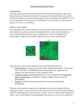
1. Understanding Raster Data
Introduction
The following document is intended to provide a basic understanding of raster data.
Raster data layers (commonly referred to as grids) are the essential data layers used in
all tools developed by the National Interagency Fuels Technology Team (NIFTT). If you
are an experienced ArcGIS user and well familiar with raster data, you may skip this
primer or review it as a refresher.
What is raster data?
In its simplest form, a raster consists of a matrix of cells (or pixels) organized into rows
and columns (or a grid), as shown in the graphic below, where each cell contains a
value representing information, such as temperature. Rasters are digital aerial
photographs, imagery from satellites, digital pictures, or even scanned maps.
Data stored in a raster format represent real‐world phenomena such as:
• Thematic data (also known as discrete data), representing features such as land‐
use or soils data. LANDFIRE data layers depicting fuels, vegetation, fire
regimes, and other features are also examples of this.
• Continuous data representing phenomena such as temperature and elevation
data or spectral data, including, for example, satellite images and aerial
photographs.
• Pictures; examples include scanned maps or drawings and building
photographs.
Thematic and continuous rasters may be displayed as data layers along with other
geographic data on a map, but they are often used as the source data for spatial analysis
with the ArcGIS Spatial Analyst extension. Picture rasters are often used as attributes in
tables—they can be displayed with geographic data and are used to convey additional
1

2. Understanding Raster Data
information about map features.
While the structure of raster data is simple, it is exceptionally useful for a wide range of
applications. Within a GIS, the uses of raster data fall under four main categories:
1) Rasters as base maps
A common use of raster data in a GIS is as a background display for other feature
layers. For example, orthophotographs displayed underneath other layers provide
the map user with confidence that map layers are spatially aligned and represent real
objects, as shown in the image below. Three main sources of raster base maps are
orthophotos from aerial photography, satellite imagery, and scanned maps.
2) Rasters as surface maps
Rasters are well suited for representing data that changes continuously across a
landscape (surface). They provide an effective method for storing the continuity as a
surface. They also provide a regularly spaced representation of surfaces. Elevation
values measured from the earthʹs surface are the most common application of surface
maps, as depicted in the graphic below. Other values, such as rainfall, temperature,
concentration, and population density, can also define surfaces that can be spatially
analyzed.
2

3. Understanding Raster Data
3) Rasters as thematic maps
Rasters representing thematic data can be derived from analyzing other data. A
common analysis application is the classification of a satellite image by land‐cover
categories. Basically, this activity groups the values of multispectral data into classes
(such as biophysical settings shown in the graphic below) and assigns a categorical
value. Thematic maps can also result from geoprocessing operations that combine
data from various sources, such as vector, raster, and terrain data. For example, a user
can process data through a geoprocessing model to create a raster data set that maps
suitability for a specific activity. Most of the LANDFIRE data layers are derived in
this manner.
4) Rasters as attributes of a feature
Rasters used as attributes of a feature may be digital photographs (see image below),
scanned documents, or scanned drawings related to a geographic object or location. A
parcel layer may have scanned legal documents identifying the latest transaction for
that parcel, or a layer representing cave openings may have pictures of the actual cave
3

4. Understanding Raster Data
openings associated with the point features.
Why store data as a raster?
Sometimes there is no choice as to how data are stored; for example, imagery may only
be available as a raster. However, there are many other features (such as points) and
measurements (such as rainfall) that could be stored as either a raster or a feature
(vector) data type.
Following is a list of the advantages of storing data as a raster:
• A simple data structure—A matrix of cells with values representing a coordinate
and sometimes linked to an attribute table
• A powerful format for advanced spatial and statistical analysis
• The ability to represent continuous surfaces and perform surface analysis
• The ability to uniformly store points, lines, polygons, and surfaces
• The ability to perform fast overlays with complex data sets
Storage space must be a consideration when working with rasters, as they can be
potentially very large data sets. Resolution increases as the size of the cell decreases;
however, cost normally also increases in both disk space and processing speeds. For a
given area, changing cells to one‐half the current size requires as much as four times the
storage space, depending on the type of data and storage techniques used. There is also
a loss of precision that accompanies restructuring data to a regularly spaced raster‐cell
boundary.
General characteristics of raster data
In raster data sets, each cell (which is also known as a pixel) has a value. The cell values
represent the phenomenon portrayed by the raster data set such as a category,
magnitude, height, or spectral value. The category could be a land‐use class such as
4

5. Understanding Raster Data
grassland, forest, or road. A magnitude might represent gravity, noise pollution, or
percent rainfall. Height (distance) could represent surface elevation above mean sea
level, which can be used to derive slope, aspect, and watershed properties. Spectral
values are used in satellite imagery and aerial photography to represent light
reflectance and color.
Cell values can be either positive or negative, integer, or floating point. Integer values
are best used to represent categorical (discrete) data, and floating‐point values to
represent continuous surfaces. All LANDFIRE data layers are stored as integer value
rasters. Cells can also have a NoData value to represent the absence of data.
A cell value applies to the center point of the cell and to the entire area of the cell, as
depicted below, depending on the raster application.
The area (or surface) represented by each cell consists of the same width and height and
is an equal portion of the entire surface represented by the raster (see graphic below).
For example, a raster representing elevation (that is, digital elevation model) may cover
an area of 100 square kilometers. If there were 100 cells in this raster, each cell would
represent one square kilometer of equal width and height (that is, 1 km x 1 km).
LANDFIRE data cells are 30 meters by 30 meters, with each cell or pixel representing an
area of 900 square meters, or .2224 acres.
5

6. Understanding Raster Data
The dimension of the cells can be as large or as small as needed to represent the surface
conveyed by the raster data set and the features within the surface, such as a square
kilometer, square foot, or even a square centimeter. The cell size determines how coarse
or fine the patterns or features in the raster will appear. The smaller the cell size, the
smoother or more detailed the raster will be. However, the greater the number of cells,
the longer it will take to process, and it will increase the demand for storage space. If a
cell size is too large, information may be lost or subtle patterns may be obscured. For
example, if the cell size is larger than the width of a road, the road may not exist within
the raster data set. In the diagram below, you can see how this simple polygon feature
will be represented by a raster data set at various cell sizes.
Raster attribute tables
Raster data sets that contain attribute tables typically have cell values that represent or
define a class, group, category, or membership. For example, a satellite image may
have undergone a classification analysis to create a raster data set that defines land uses.
Some of the classes in the land‐use classification may be forest land, wetland, crop land,
and urban. The numbers below could represent which cell value in the raster data set
would define the land use:
6

7. Understanding Raster Data
1 Forest land
2 Wetland
3 Crop land
4 Urban
By building a raster attribute table, you can maintain this tableʹs attribute information
with this classified raster data set, as well as define additional fields to be stored in it.
For example, there may be specific codes associated with those classes or further
descriptions of what those classes represent. You may also want to perform
calculations on the information in the table. For example, you may want to keep
records of the total area represented by those classes by calculating the number of cells
multiplied by the area each cell represents. You can also join the raster attribute table to
other tables.
The graphic below illustrates a raster data set with attribute table. The NoData values
are not calculated in the raster attribute table. There are also three columns that are
calculated by default; the other columns can be added individually or by using a join
operation.
When a raster attribute table is generated, there are three default fields created in the
table: OID, VALUE, and COUNT. It is not possible to edit the content in these fields.
The ObjectID (OID) is a unique system‐defined object identifier number for each row in
the table. VALUE is a list of each unique cell value in the raster data sets. COUNT
represents the number of cells in the raster data set with the cell value in the VALUE
column. Cell values represented by NoData are not calculated in the raster attribute
table.
In summary, understanding the structure and function of raster data is an important
foundation for working with LANDFIRE data and the suite of NIFTT tools. For
7

8. Understanding Raster Data
additional information regarding raster data, please consult ArcGIS Desktop Help or
visit the ESRI support web site at support.esri.com.
Portions of this work include the intellectual property of ESRI and are used herein under license. Aspects
of the ArcGIS® Desktop Help text and graphics have been used and edited for training purposes by
Acadia West LLC. Copyright © 2009 ESRI. All rights reserved.
8