Is curve derivation

1
CHAPTER 10CHAPTER 10 Aggregate Demand IAggregate Demand I slide 20
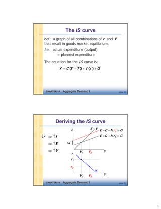
TheThe ISIS curvecurve
def: a graph of all combinations of r and Y
that result in goods market equilibrium,
i.e. actual expenditure (output)
= planned expenditure
The equation for the IS curve is:
( ) ( )Y C Y T I r G= − + +
Y2Y1
Y2Y1
Deriving theDeriving the ISIS curvecurve
↓r ⇒ ↑I
Y
E
r
Y
E =C +I(r1 )+G
E =C +I(r2 )+G
r1
r2
E =Y
IS
ΔI⇒ ↑E
⇒ ↑Y

2
Understanding theUnderstanding the ISIS curve’s slopecurve’s slope
The IS curve is negatively sloped.
Intuition:
A fall in the interest rate motivates firms to
increase investment spending, which drives
up total planned spending (E ).
To restore equilibrium in the goods market,
output (a.k.a. actual expenditure, Y ) must
increase.
The ISThe IS curve and the Loanable Funds modelcurve and the Loanable Funds model
S, I
r
I(r )
r1
r2
r
YY1
r1
r2
(a) The L.F. model (b) The IS curve
Y2
S1S2
IS

3
Fiscal Policy and theFiscal Policy and the ISIS curvecurve
We can use the IS-LM model to see
how fiscal policy (G and T ) can affect
aggregate demand and output.
Let’s start by using the Keynesian Cross
to see how fiscal policy shifts the IS
curve…
Y2Y1
Y2Y1
Shifting theShifting the ISIS curve:curve: ΔΔGG
At any value of r,
↑G ⇒ ↑E ⇒ ↑Y
Y
E
r
Y
E =C +I(r1 )+G1
E =C +I(r1 )+G2
r1
E =Y
IS1
The horizontal
distance of the
IS shift equals
IS2
…so the IS curve
shifts to the right.
1
1 MPC
Y GΔ = Δ
−
ΔY

4
Exercise: Shifting the IS curveExercise: Shifting the IS curve
Use the diagram of the Keynesian Cross
or Loanable Funds model to show how
an increase in taxes shifts the IS curve.
The Theory of Liquidity PreferenceThe Theory of Liquidity Preference
due to John Maynard Keynes.
A simple theory in which the interest rate
is determined by money supply and
money demand.

5
Money SupplyMoney Supply
The supply of
real money
balances
is fixed:
( )
s
M P M P=
M/P
real money
balances
r
interest
rate
( )
s
M P
M P
Money DemandMoney Demand
Demand for
real money
balances:
M/P
real money
balances
r
interest
rate
( )
s
M P
M P
( ) ( )
d
M P L r=
L(r)

6
EquilibriumEquilibrium
The interest
rate adjusts
to equate the
supply and
demand for
money:
M/P
real money
balances
r
interest
rate
( )
s
M P
M P
( )M P L r= L(r)
r1
How the Fed raises the interest rateHow the Fed raises the interest rate
To increase r,
Fed reduces M
M/P
real money
balances
r
interest
rate
1M
P
L(r)
r1
r2
2M
P

7
CASE STUDYCASE STUDY
Volcker’sVolcker’s Monetary TighteningMonetary Tightening
Late 1970s: π > 10%
Oct 1979: Fed Chairman Paul Volcker
announced that monetary policy
would aim to reduce inflation.
Aug 1979-April 1980:
Fed reduces M/P 8.0%
Jan 1983: π = 3.7%
How do you think this policy change
would affect interest rates?
How do you think this policy changeHow do you think this policy change
would affect interest rates?would affect interest rates?
Volcker’sVolcker’s Monetary Tightening,Monetary Tightening, cont.cont.
Δi < 0Δi > 0
1/1983: i = 8.2%
8/1979: i = 10.4%
4/1980: i = 15.8%
flexiblesticky
Quantity Theory,
Fisher Effect
(Classical)
Liquidity Preference
(Keynesian)
prediction
actual
outcome
The effects of a monetary tightening
on nominal interest rates
prices
model
long runshort run

8
The LM curveThe LM curve
Now let’s put Y back into the money demand
function:
( , )M P L r Y=
The LM curve is a graph of all combinations of
r and Y that equate the supply and demand
for real money balances.
The equation for the LM curve is:
( )
d
M P L r Y= ( , )
Deriving the LM curveDeriving the LM curve
M/P
r
1M
P
L(r,Y1 )
r1
r2
r
YY1
r1
L(r,Y2 )
r2
Y2
LM
(a) The market for
real money balances
(b) The LM curve

9
Understanding theUnderstanding the LMLM curve’s slopecurve’s slope
The LM curve is positively sloped.
Intuition:
An increase in income raises money
demand.
Since the supply of real balances is fixed,
there is now excess demand in the money
market at the initial interest rate.
The interest rate must rise to restore
equilibrium in the money market.
HowHow ΔΔMM shifts the LM curveshifts the LM curve
M/P
r
1M
P
L(r,Y1 )
r1
r2
r
YY1
r1
r2
LM1
(a) The market for
real money balances
(b) The LM curve
2M
P
LM2

10
Exercise: Shifting the LM curveExercise: Shifting the LM curve
Suppose a wave of credit card fraud
causes consumers to use cash more
frequently in transactions.
Use the Liquidity Preference model
to show how these events shift the
LM curve.
The shortThe short--run equilibriumrun equilibrium
The short- run equilibrium is
the combination of r and Y
that simultaneously satisfies
the equilibrium conditions in
the goods & money markets:
( ) ( )Y C Y T I r G= − + +
Y
r
( , )M P L r Y=
IS
LM
Equilibrium
interest
rate
Equilibrium
level of
income

11
The Big PictureThe Big Picture
Keynesian
Cross
Theory of
Liquidity
Preference
IS
curve
LM
curve
IS-LM
model
Agg.
demand
curve
Agg.
supply
curve
Model of
Agg.
Demand
and Agg.
Supply
Explanation
of short-run
fluctuations
Chapter summaryChapter summary
1. Keynesian Cross
basic model of income determination
takes fiscal policy & investment as exogenous
fiscal policy has a multiplied impact on income.
2. IS curve
comes from Keynesian Cross when planned
investment depends negatively on interest rate
shows all combinations of r and Y that
equate planned expenditure with actual
expenditure on goods & services

12
3. Theory of Liquidity Preference
basic model of interest rate determination
takes money supply & price level as exogenous
an increase in the money supply lowers the
interest rate
4. LM curve
comes from Liquidity Preference Theory when
money demand depends positively on income
shows all combinations of r andY that equate
demand for real money balances with supply
5. IS-LM model
Intersection of IS and LM curves shows the
unique point (Y, r ) that satisfies equilibrium
in both the goods and money markets.

13
Preview of Chapter 11Preview of Chapter 11
In Chapter 11, we will
use the IS-LM model to analyze the impact
of policies and shocks
learn how the aggregate demand curve
comes from IS-LM
use the IS-LM and AD-AS models together
to analyze the short-run and long-run
effects of shocks
learn about the Great Depression using our
models

Is curve derivation

Recommended

Recommended

More Related Content

What's hot

What's hot (20)

Viewers also liked

Viewers also liked (14)

Similar to Is curve derivation

Similar to Is curve derivation (20)

Recently uploaded

Recently uploaded (20)

Is curve derivation