1. General phenological model to characterise the timing of
flowering and veraison of Vitis vinifera L._140 206..216
A.K. PARKER1
*, I.G. DE CORTÁZAR-ATAURI2†
, C. VAN LEEUWEN1
and I. CHUINE2
1
ENITA, Bordeaux University, UMR EGFV, ISVV, 1 Cours du Général de Gaulle, CS 40201, 33175,
Gradignan-Cedex, France
2
Centre d’Ecologie Fonctionelle et Evolutive, Equipe Bioflux, CNRS, 1919 Route de Mende, 34293 Montpellier
Cedex 5, France
Present addresses: * Marlborough Wine Research Centre, 85 Budge St, PO Box 845, Blenheim 7240, New Zealand.
†
European Commission JRC-IPSC-MARS-Agri4cast action, via E. Fermi 2749 – TP483, I-21027 Ispra (VA), Italy.
Corresponding author: Miss Amber K. Parker, fax +64-3-984-4311, email amber.parker@lincolnuni.ac.nz
Abstract
Background and Aims: Phenological models, which are based on responses of the plant to temperature, are useful
tools to predict grapevine (Vitis vinifera L.) phenology in various climate conditions. This study aimed to develop a
single process-based phenological model at the species level to predict two important stages of development for V.
vinifera L.: flowering and veraison.
Methods and Results: Three different phenological models were tested and the model that gave the best results
was optimised for its parameters. The chosen model Spring Warming was found optimal with regard to the trade-off
between parsimony of input parameters and efficiency. The base temperature (Tb) of 0°C calculated from the 60th
day (t0) of the year (for the Northern hemisphere) was found to be the most optimal parameter set tested. This model
henceforth referred to as the Grapevine Flowering Veraison model (GFV) was successfully validated at the varietal
level using an independent dataset.
Conclusions: A general phenological model, GFV, has been successfully developed to characterise the timing of
flowering and veraison for the grapevine.
Significance of the Study: The model is simple for the user, can be successfully applied to many varieties and can
be used as an easy predictor of phenology for different varieties under climate change scenarios.
Keywords: flowering, modelling, phenology, temperature, veraison
Introduction
Several studies have highlighted the impact of climate change
on the timing of seasonal activities in plants and animals such as
the advancement of the phenological stages of flowering and
leaf unfolding (Menzel and Fabian 1999, Menzel 2003, Cleland
et al. 2007). As with other plants, temperature and photoperiod
are considered to be fundamental in influencing grapevine (Vitis
vinifera L.) phenological development and ripening (Winkler
et al. 1962, Huglin 1978, Jones and Davis 2000, Jones 2003,
Jones et al. 2005, Van Leeuwen et al. 2008, Duchêne et al.
2010). Forecasted increases in temperatures are predicted to
cause earlier development and therefore a general advancement
of grapevine phenological stages (Duchêne and Schneider 2005,
Jones et al. 2005, Webb et al. 2007, Petrie and Sadras 2008,
Duchêne et al. 2010). The overall effect predicted for climate
change is a shortening of the growth season with maturation
occurring during hotter periods of the year (Webb et al. 2007,
Hall and Jones 2009, Duchêne et al. 2010).
When the vegetative and reproductive development of the
grapevine are well adapted to the local conditions, the grapes at
harvest may correspond to a desired combination of sugar,
acidity, aromatic and phenolic profile or other desired qualities
for the production of high-quality wine (Jones and Davis 2000,
Jones et al. 2005, Jones 2006, Van Leeuwen et al. 2008). Grapes
which ripen in the warmest part of the summer contain less
aromas or aroma precursors (Van Leeuwen and Seguin 2006).
As a result of the predicted climate changes, it is possible that
varieties currently planted under certain climate conditions
today may no longer be adapted to reach maturity under the
same conditions in the future. Therefore, understanding how
temperature influences the timing of V. vinifera L. vegetative and
reproductive development as well as identifying varietal specific
differences in phenology and maturity is crucial.
Up until now, process-based phenological models for the
grapevine work on the assumption that phenological develop-
ment is mainly regulated by temperature (Williams et al.
1985a,b; Villaseca et al. 1986, Moncur et al. 1989, Riou 1994,
Oliveira 1998, Jones 2003, Van Leeuwen et al. 2008; García de
Cortázar-Atauri et al. 2009; Caffarra and Eccel 2010, Duchêne
et al. 2010, Nendel 2010). These models are driven by a tem-
perature summation from a defined date and above a minimum
temperature (threshold) until the appearance of a phenological
stage (often judged at 50% level of appearance). Classically, the
Spring Warming (SW) model (also known as Growing Degrees
Days (GDD)) is the simplest model used to estimate grapevine
phenology (bud break, flowering and veraison). This model
calculates a summation of daily heat requirements calibrated
from a base temperature (usually 10°C for grapevine) and from
206 Grapevine flowering and veraison model Australian Journal of Grape and Wine Research 17, 206–216, 2011
doi: 10.1111/j.1755-0238.2011.00140.x
© 2011 Australian Society of Viticulture and Oenology Inc.

2. a given date. The sum of the resulting values gives a measure of
the state of forcing (heat requirements) in degrees days (°C.d).
More complex phenological models also take into account chill
requirements (in addition to heat requirements) necessary to
break dormancy (for a review see Chuine et al. 2003). Such
models have been successfully adapted for other species (Bidabe
1965a,b; Chuine 2000, Cesaraccio et al. 2004, Crepinsek et al.
2006). Recently, phenological models have been successfully
developed for the bud break stage of the grapevine, which
incorporate both chill and heat units (García de Cortázar-Atauri
et al. 2009; Caffarra and Eccel 2010).
Process-based modelling techniques aim to achieve tempo-
ral and spatial robustness; i.e. the difference between years and
regions in the date of a phenological event for a variety can be
explained solely by the differences in abiotic factors such as
temperature and photoperiod (Chuine et al. 2003). Such tech-
niques have not been fully explored for flowering and veraison
of grapevines. Furthermore, the parameter estimates defining
existing indices have not been considered with respect to
current modelling capabilities and the availability of new data-
bases. For example, the relevance of the base temperature
parameter of 10°C, which was defined by Winkler et al. (1962)
for grapevines in California, and often applied in other vine-
yards and regions has been questioned in prior studies (Moncur
et al. 1989, Oliveira 1998, Duchêne et al. 2010) and has not
been tested on larger databases (covering more regions and time
periods) using more modern and efficient optimisation algo-
rithms for model parameterisation.
The aim of this study was to develop a simple process-based
phenological model to predict two important stages of develop-
ment of V. vinifera L., namely flowering and veraison. The best
model was selected in terms of efficiency relative to its complex-
ity. The developed model aimed to convey temporal and spatial
robustness for the species V. vinifera L. By using this approach, all
varieties can be compared within the same modelling frame-
work and the model can be applied across different locations.
The model can be parameterised further to describe the timing
of flowering and veraison for individual varieties.
Materials and methods
Phenological data
Historical data for 50% flowering and 50% veraison were
collected from scientific research institutes, extension services
(‘Chambres d’Agriculture’) and private companies in France,
Italy, Switzerland and Greece. Dates of 50% flowering were
defined as the date when 50% of flowers reached the stage
of anthesis, identified as stage 23 on the modified Eichorn
and Lorenz (E-L) scale (Coombe 1995). Dates of 50% veraison
corresponded to the onset of the ripening period identified as
the date when 50% of berries softened or changed from green
to translucent for white varieties, or a change of colour of
50% of berries for red varieties (stage 35 on the modified E-L
scale).
The phenological observations collected for this study
spanned from 1960 to 2007, from 123 different locations (pre-
dominantly in France). The observations corresponded to 81
varieties, 2278 flowering observations and 2088 veraison obser-
vations (Table 1). Although spanning 55 years, most data col-
lected corresponded to the last 10 years for both phenological
stages (Figure 1). Geographically, the data covered 12 of the
principal viticultural regions of France, Changins in Switzer-
land, Veneto and Tuscany in Italy, and the Peloponnese region
in Greece. These observations were not collected all at the same
time. The first set of observations collected was used to param-
eterise the models. After model selection, a second set of obser-
vations was collected to validate the models. The validation data
used corresponded to 11 varieties, 424 observations for veraison
and 440 observations for flowering.
Temperature data
Daily minimum and maximum temperatures were collected
from meteorological stations situated not more than 5 km
away and within ⫾100 m in altitude for each phenological
data site. The average daily temperature was calculated as
the arithmetic mean of the daily maximum and minimum
temperature.
Phenological models
Three different process-based models were tested: (i) SW with
two different forms, (ii) UniFORC and (iii) UniCHILL (Chuine
2000, Chuine et al. 2003).
Spring Warming and UniFORC consider only the action of
forcing temperatures. These models assume a phenological stage
occurs where ts corresponds to the day when a critical state of
forcing Sf, denoted F* has been reached (Eqn 1):
S t R x F
t
t
f s f t
s
*
( ) ( )
= ≥
∑
0
(1)
The state of forcing is described as a daily sum of the rate of
forcing, Rf, which starts at t0 (day of the year, DOY) and xt is the
daily mean temperature. The rate of forcing in the SW model is
defined by Eqn 2:
R x GDD x
x Tb
x Tb x Tb
f t t
t
t t
if
if
( ) ( )
= =
<
− ≥
⎧
⎨
⎩
0
(2)
The SW model contains three parameters, t0, Tb and F*, where
Tb corresponds to a base temperature above which the thermal
summation is calculated.
First, the t0 value was forced as 1 January, and Tb and F*
were fitted parameters. This corresponds to what is normally
considered the GDD model for grapevine except the base tem-
perature was not forced a priori to 10°C but was fitted to the
data.
Second, t0 was left unforced; therefore, t0, Tb and F* were
fitted parameters.
Rate of forcing in the UniFORC model is defined by Eqn 3:
R x
x
e
x
d x e
f t
t
t
if
if
t
( )
( )
=
<
+
≥
⎧
⎨
⎪
⎩
⎪ −
0 0
1
1
0
(3)
The UniFORC model contains four parameters where t0 is
forced as 1 January and d, e and F* are fitted, with d < 0 and
e > 0.
The third model that was tested, UniCHILL, considers in
addition to the UniFORC model, the action of chilling tempera-
tures involved during the dormancy period. It assumes a critical
state of chilling (Sc) C* (Eqn 4) must be reached to break dor-
mancy (td), with the rate of development of chilling (Rc) defined
by Eqn 5. At this point, a sum of forcing units can start to
accumulate until this reaches a critical state F* as described by
Eqn 3. The UniCHILL model has seven fitted parameters a, b, c,
C*, pertaining to the chilling function (Eqn 5) and d, e, F*,
Parker et al. Grapevine flowering and veraison model 207
© 2011 Australian Society of Viticulture and Oenology Inc.

3. Table
1.
Quantity
and
description
of
data
by
country,
region,
number
of
sites,
years
and
varieties
for
flowering
and
veraison
observations
collected
in
the
database.
Country
Region
Number
of
sites
Flowering
Veraison
Varieties
Years
n
Years
n
France
Alsace
1
1976–1986
1988–2001
156
1976–1986
1988–2001
154
Cabernet-Sauvignon,
Chardonnay,
Chasselas,Grenache
noir,
Merlot,
Pinot
noir,
Riesling,
Syrah,
Ugni
blanc
Champagne
3
1998–2005
38
1998–2004
34
Chardonnay,
Pinot
noir
Loire
Valley
15
1981–2007
338
1982–1990
1992–2000
2002–2007
178
Cabernet
franc,
Cabernet-Sauvignon,
Chardonnay,
Chasselas,
Chenin,
Cot,
Gamay,
Grenache
noir,
Groulleau,
Pinot
noir,
Riesling,
Sauvignon
blanc,
Syrah,
Ugni
blanc
Burgundy
7
1994–2006
105
2004–2005
2
Chardonnay,
Gamay,
Pinot
noir
Beaujolais
4
1992–2007
45
1992–2007
43
Gamay
Rhone
1
2000–2007
8
2000–2007
8
Syrah
Languedoc-
Roussillon
27
1960
1962–1966
1979–1982
1986–2007
695
1962–1964
1976–1985
1987–2007
729
Altesse,
Arinarnoa,
Bourboulenc,
Cabernet
franc,
Cabernet-Sauvignon,
Caladoc,
Carignan
noir,
Chardonnay,
Chasselas,
Chenanson,
Chenin,
Cinsaut,
Colombard,
Cot,
Egiodola,
Ekigaina,
Gamay,
Gewürztraminer,
Gouais
blanc,
Grenache
noir,
Jacquère,
Marsalan,
Marsanne,
Merlot,
Mondeuse,
Mourvèdre,
Muscadelle,
Muscat
blanc
à
pétits
grains,
Muscat
of
Alexandria,
Nebbiolo,
Petit
verdot,
Pinotage,
Pinot
gris,
Pinot
noir,
Pinot
meunier,
Piquepoul
blanc,
Piquepoul
noir,
Poulsard
Portan,
Riesling,
Roussanne,
Sangiovese,
Sauvignon
blanc,
Savagnin,
Segalin,
Sémillon,
Syrah,
Tannat,
Tempranillo,
Trousseau,
Ugni
blanc,
Vermentino,
Viognier,
Xinomavro,
Zweigelt
blau
Bordeaux
9
1974–2007
126
1961–1971
1973–2007
215
Cabernet
franc,
Cabernet-Sauvignon,
Merlot,
Muscadelle,
Sauvignon
blanc,
Sémillon
Mid-Pyrénées
4
1999–2004
22
1999–2004
22
Colombard
Provence-Alpes
-Cote
d’Azur
45
1976–1977
1979–1980
1982
1984–1986
1994
1997–2007
162
1997–2007
88
Alicante
bouschet,
Carignan
noir,
Chason,
Cinsaut,
Grenache
blanc,
Grenache
noir,
Merlot,
Mourvèdre,
Muscat
of
Hamburg,
Syrah
Corsica
1
—
—
1998–2006
27
Sangiovese,
Sciaccarello,
Vermentino
Greece
Peloponnese
3
1997–1998
6
1997–1998
6
Agiorgitiko
Switzerland
Changins
1
1991–1999
337
1991–1999
338
Aligoté,
Amigne,
Arvine,
Bondola,
Cabernet
franc,
Cabernet-Sauvignon,
Chardonnay,
Charmont,
Chasselas,
Cornalin,
Diolmoir,
Doral,
Gamaret,
Garanoir,
Gewürztraminer,
Grenache
noir,
Humagne
blanc,
Humagne
rouge,
Kerner,
Marsanne,
Merlot,
Mourvèdre,
Muscat
blanc
à
pétits
grains,
Nebbiolo,
Pinot
blanc,
Pinot
cortaillod,
Pinot
gris,
Pinot
mariafield,
Rauschling,
Riesling,
Sangiovese,
Sauvignon
blanc,
Savagnin,
Sémillon,
Sylvaner,
Syrah,
Ugni
blanc
Italy
Veneto
Tuscany
2
1964–1981
1985–2006
240
1964–1981
1984–2006
244
Arinarnoa,
Cabernet
franc,
Cabernet-Sauvignon,
Chardonnay,
Merlot,
Petit
verdot,
Pinot
noir,
Sangiovese,
Sauvignon
blanc,
Ugni
blanc
Total
123
2278
2088
81
varieties
Not
all
varieties
are
present
for
both
flowering
and
veraison
within
a
given
region;
new
crosses
(unnamed)
are
not
listed
under
varieties
(although
the
data
is
included
in
the
observations,
site
and
years).
n
corresponds
to
the
total
number
of
observations
for
each
phenological
stage
within
a
region.
208 Grapevine flowering and veraison model Australian Journal of Grape and Wine Research 17, 206–216, 2011
© 2011 Australian Society of Viticulture and Oenology Inc.

4. pertaining to the forcing function. t0 is fixed at 1 September for
Sc such that
S t R x C
t
t
c d c t
d
*
( ) ( )
= ≥
∑
0
(4)
and
R x
ea x c b x c
c t
t t
( )
( ) ( )
=
+ − + −
1
1
2 (5)
Model parameterisation and selection
All data for flowering and veraison across all varieties from the
parameterisation dataset were used to fit the most accurate
model of the timing of flowering and veraison at the species
level. Model parameters were fitted using the simulated
annealing algorithm of Metropolis following Chuine et al.
(1998). The best model was selected based on three criteria: (i)
the model with the highest efficiency, i.e. that gives the
highest percentage of variance explained (EF; Greenwood
et al. 1985; Eqn 6) where a negative value indicated that the
model performed worse than the null model (mean date of
flowering or veraison), and a value above zero indicated that
the model explained more variance than the null model (with
a maximum value of 1); (ii) the root means squared error
(RMSE; Eqn 7), which gives the mean error of the prediction
in days; (iii) the Akaike Information Criterion (AIC; Burnham
and Anderson 2002; Eqn 8), which rates models in terms of
parsimony and efficiency, where the lowest value is associated
with the best model.
EF
i i
i
i
i
= −
−
−
⎛
⎝
⎜
⎜
⎜
⎜
⎞
⎠
⎟
⎟
⎟
⎟
=
=
∑
∑
1
2
1
2
1
( )
( )
S O
O O
n
n (6)
RMSE
i i
i
=
−
=
∑( )
S O
n
n
2
1
(7)
AIC
i i
i
= ×
−
⎛
⎝
⎜
⎜
⎞
⎠
⎟
⎟ +
=
∑
n
S O
n
k
n
ln
( )2
1
2 (8)
where Oi is the observed value, Si is the simulated value, Ō is the
mean observed value of the dataset used, n is the number of
observations, k is the number of parameters.
Once a model was selected, the parameter estimates were
optimised in order to fix parameters (excluding F*) to the same
values for all varieties and both flowering and veraison stages.
Model validation
The selected model was validated for the most frequently rep-
resented varieties (11 in total) for which supplementary inde-
pendent data had been obtained after model parameterisation.
Prior validation, the F* values of the selected model were fitted
for flowering and veraison for each of the 11 varieties from the
parameterisation data; these values were validated with the
validation data using the statistical criterion of EF and RMSE.
Results
Model selection
The four model types (two versions of SW, UniFORC,
UniCHILL) were compared for the same number of observa-
tions, i.e. 1033 observations for flowering and 925 observations
for veraison. Overall, there was very little difference between
UniFORC, UniCHILL and SW in terms of efficiency (Table 2).
However, the SW model (all parameters fitted) was more effi-
cient than any of the other models for both flowering and
veraison as indicated by the EF and RMSE values. The lower
AIC values obtained for the SW model with unfixed parameters
for both flowering and veraison indicated that SW was the best
model with regard to the trade-off between parsimony and
efficiency. SW using the classical parameter value of 1 January
as t0 was the least efficient model overall. The SW model with
unfixed parameters for t0 and Tb was subsequently chosen for
our study.
Optimisation of a single model for flowering and veraison
More data from the parameterisation dataset could be used to fit
the SW model, which unlike the UniCHILL model does not
require temperature data prior to 1 January. The UniCHILL
Year
1950 1960 1970 1980 1990 2000 2010
Number
of
observations
0
20
40
60
80
100
120
140
160
Flowering
Veraison
Figure 1. Distribution of phenology data by year for the complete
phenological database of flowering and veraison. Closed circles (䊉)
represent flowering data; open circles (䊊) represent veraison data.
Table 2. Statistical analysis of the four tested models for
flowering and veraison using the same dataset.
Model: SW SW t0 = 1 January UniFORC UniCHILL
Flowering
EF 0.80 0.75 0.76 0.79
RMSE 5.4 6.1 6.0 5.6
AIC 3481 3740 3709 3559
Veraison
EF 0.74 0.57 0.72 0.69
RMSE 8.0 10.2 8.2 8.7
AIC 3845 4299 3909 4018
1033 observations for flowering and 925 observations for veraison were used.
SW refers to the model Spring Warming; EF is the efficiency of the model; RMSE
is the root means squared error; AIC is the Akaike Information Criterion.
Parker et al. Grapevine flowering and veraison model 209
© 2011 Australian Society of Viticulture and Oenology Inc.

5. model requires temperature data from 1 September of the prior
year as it describes the action of temperature on the dormancy
phase. The SW model was fitted again with 1092 flowering
observations and 980 veraison observations. The best estimates
of parameters t0 and Tb for the SW model fitted on flowering
dates were 56.4 days and 2.98°C, respectively (Table 3). For the
sake of simplicity for users, these values were rounded to
60 days and 3°C without altering the efficiency of the model for
flowering. When applied to veraison, the parameter estimates of
60 days and 3°C slightly decreased the model efficiency (0.70 vs
0.72) compared to the parameter estimates fitted on veraison
dates. Conversely, the parameter estimates of t0 at 92 days and a
Tb value of 4°C fitted for veraison dates greatly reduced the
efficiency of the model for flowering compared to the parameter
values obtained for fitting the model to flowering dates (0.79 vs
0.71). Since our aim was to develop one model that could be
used for a diverse range of varieties for the timing of appearance
of these two phenological stages, we looked for parameter esti-
mates that could therefore optimise the efficiency of the verai-
son model without unduly altering the efficiency of the model
for predicting flowering. Further fitting of veraison (Table 3) by
maintaining t0 at 60 days yielded a Tb estimate of 0°C, increasing
the efficiency of the veraison model slightly (0.72 vs 0.70) and
reducing slightly the efficiency of the flowering model (0.76
compared vs 0.79). A greater range of values for parameters t0
and Tb were then investigated to further confirm the choice of
initial parameter estimates that were optimised for the veraison
model (t0 value of 60 days, Tb value of 0°C). The efficiency of the
model did increase as t0 increased from 0 to 60 days (Tb at 0°C)
after which the efficiency remained stable (Figure 2); a decrease
in the efficiency of the model occurred when Tb increased from
0°C to 15°C (t0 at 60 days; Table 4). This confirmed the choice of
estimates for parameters t0 and Tb following the optimisation
procedure. The model SW using the new parameter estimates of
60 days for t0 and a Tb value of 0°C was slightly more efficient
for flowering than the classical model of SW (GDD) with the
parameters t0 at 1 day and a Tb value of 10°C. The new model
was substantially more efficient for veraison (Table 5).
Gladstones (1992) suggested that phenology predicted by
the temperature summation method of GDD was improved
when the average temperature was capped at 19°C. That is, for
every average daily temperature greater than 19°C, the value of
19 replaces the actual average in the calculation of the thermal
summation. We tested this hypothesis for the model SW with t0
at 60 days and Tb fitted, by limiting the maximum average
temperature value used in the model between the values of
15°C and 25°C. This resulted in a decreased efficiency of the
t0 (DOY)
0 20 40 60 80 100
EF
0.50
0.55
0.60
0.65
0.70
0.75
Figure 2. Change in the efficiency (EF) of veraison model (Spring
Warming, Tb value of 0°C) in response to changes in t0.
Table 3. Efficiency of the Spring Warming model to predict flowering and veraison for different
sets of parameter estimates of t0 and Tb (F* is adjusted for each stage).
Parameters t0 (d) Tb (°C) Flowering Veraison
t0 and Tb fitted on flowering dates 56 3 0.79 0.69
t0 and Tb fitted on veraison dates 92 4 0.71 0.72
t0 and Tb fixed 60 3 0.79 0.70
t0 and Tb fixed 60 0 0.76 0.72
1092 observations were used for flowering and 980 observations were used for veraison.
Table 4. Statistical analysis of the optimisation process
for Tb for veraison using the model Spring Warming t0 at
60 days.
Tb (°C)
0 3 5 7 10 12 15
EF 0.72 0.70 0.66 0.58 0.26 -0.55 -2.17
RMSE 8.14 8.40 9.00 9.90 13.17 19.09 27.35
EF is the efficiency of the model; RMSE is the root means squared error.
Table 5. Comparison of efficiency and quality of predic-
tion of flowering and veraison between the new Spring
Warming model (New SW) parameters (t0 at 60 days, Tb
of 0°C) and the classical Spring Warming model (Classical
SW) parameters (t0 at 1 day, Tb of 10°C).
Flowering Veraison
New SW Classical SW New SW Classical SW
t0 60 1 60 1
Tb 0°C 10°C 0°C 10°C
EF 0.76 0.73 0.72 0.14
RMSE 5.9 6.3 7.7 14.3
1092 observations were used for flowering; 980 observations were used for
veraison.
210 Grapevine flowering and veraison model Australian Journal of Grape and Wine Research 17, 206–216, 2011
© 2011 Australian Society of Viticulture and Oenology Inc.

6. model for any value of the maximum possible average tempera-
ture (Figure 3). The suggestion by Gladstone (1992) was there-
fore not incorporated into our model and daily average
temperatures remained uncapped.
Spring Warming with a base temperature (Tb) of 0°C calcu-
lated from the 60th day (t0) of the year was therefore selected as
the best model. This model is referred to as the Grapevine
Flowering Veraison model (GFV) from hereon.
Model validation
For both flowering and veraison, it was observed that the dis-
persion of data was similar between the data used to parameter-
ise and validate the model on a varietal level (Figures 4,5).
However, flowering was, in general, less dispersed for both the
model parameterisation and validation compared with veraison.
When the model was tested for each variety (EF values in
Tables 6,7), in general, the efficiencies were higher than that
obtained for the species (the combined cultivar values, EF of
0.76 for flowering, and 0.72 for veraison in Table 3).
For flowering, the efficiencies obtained with the validation
dataset for the 11 varieties were always greater than that of the
null model (average date). In general, the efficiency was as
expected, higher with the parameterisation dataset than with
the validation dataset given that the F* value used for the
validation process was estimated from the data used for model
parameterisation. However, for most varieties (7 out of 11), the
loss of efficiency was less than 20%. Notably, the efficiency of
the Chardonnay, Merlot, Grenache and Syrah models was not
decreased by more than 10% with the independent validation
data compared to the parameterisation data (Table 6). The
quality of prediction for each variety (RMSE) remained compa-
rable between both the parameterisation data and the validation
data. However, less data were used for the validation process.
Regardless, the RMSE values were less than 1 week for all
varieties for model parameterisation and validation.
For veraison, four varieties had less than a 20% reduction in
efficiency with the validation data (Table 7). For Cabernet franc,
Cabernet-Sauvignon, Chardonnay and Riesling, the model still
simulated veraison better than the null model (average date).
For Chasselas and Pinot noir, negative efficiencies were
obtained; however, fewer observations were used correspond-
ing to a reduced spatial and temporal representation for these
varieties. Although there were more observations for Ugni blanc
than for Chasselas and Pinot noir, a negative EF was obtained
for Ugni blanc model validation. This could be attributed to the
larger sum of squares (data not shown) between the prediction
and observation values for the validation dataset. The quality of
prediction (RMSE) was similar for all varieties for the param-
eterisation data with a maximum value of 7.81 days; the quality
was slightly less for the validation data with a maximum value
obtained of 9.79 days. However, for most varieties (10 out of
11), there was a difference of less than 3 days between the
RMSE for the parameterisation and validation data.
Discussion
Relevance of the GFV model for grapevine
We modelled flowering and veraison using process-based
models (Chuine et al. 2003) so far untested for the grapevine
with the aim of developing the simplest model possible at the
species level. The proposed model GFV with a start date of the
60th DOY (t0) for application in the Northern Hemisphere; and
base temperature, Tb, of 0°C showed the best overall perfor-
mance, representing the best balance between complexity and
performance compared to the other possible model choices. The
model UniCHILL, which takes into account the effect of chilling
temperature during the ‘dormancy phase’ to break bud rest, was
no more efficient or parsimonious, although it may represent a
more realistic model in terms of temperature influences during
development (García de Cortázar-Atauri et al. 2009). However,
for the purpose of a general model, the results show that flow-
ering and veraison can be predicted with good precision based
solely on the basis of heat units.
The GFV model proved more efficient than the current
classic model of GDD using a base temperature of 10°C from 1
January (in the Northern hemisphere). The base temperature
of 10°C has been proposed to represent a threshold above
which physiological processes are of importance for phenologi-
cal development. Our results indicate that either physiological
processes influencing phenological development below 10°C
could be of more importance than currently thought and/or
that the threshold temperature that is optimal for model pre-
diction is not necessarily the temperature threshold for the
underlying physiological processes of the developmental stage.
The base temperature of 0°C has the advantage for model users
in that it is simpler to calculate during the growing season
when minimum temperatures are less likely to drop below
0°C. Therefore, in such cases, its application represents a
simple addition of accumulated daily average temperatures
(from the 60th DOY).
Notably, a recent model successfully adapted to simulate
grapevine bud break in cool European regions (Nendel 2010)
used the same parameter values for the base temperature and
start day for the thermal summation (t0 at 60 days and Tb value
of 0°C) that were found optimal in this study. Given that the
datasets used and the optimisation processes differed between
this study and that of Nendel (2010), this agreement of param-
eter values indicates a convergence of different phenological
stages to the same thermal summation model. Other studies
(Williams et al. 1985b, Duchêne et al. 2010) have also proposed
initial dates very close to this proposed value of 60 days (20
February and 15 February, respectively). However, to our
knowledge, this study is the first to test and confirm the perti-
nence of this value for a dataset containing such a wide range of
varieties, locations and years for flowering and veraison. The
parameter values are to be further tested in the future for
Southern hemisphere data (where the t0 is equivalent to the
242nd DOY).
14 16 18 20 22 24 26
EF
0.62
0.64
0.66
0.68
0.70
0.72
0.74
Temperature threshold (°C)
Figure 3. The effect of capping the maximum temperature on model
efficiency (EF) for Spring Warming, t0 at 60 days.
Parker et al. Grapevine flowering and veraison model 211
© 2011 Australian Society of Viticulture and Oenology Inc.

7. (a) Cabernet franc
Observation (DOY)
100 120 140 160 180 200 220 240
Prediction
(DOY)
100
120
140
160
180
200
220
240
(b) Cabernet-Sauvignon
Observation (DOY)
100 120 140 160 180 200 220 240
Prediction
(DOY)
100
120
140
160
180
200
220
240
(c) Chardonnay
Observation (DOY)
100 120 140 160 180 200 220 240
Prediction
(DOY)
100
120
140
160
180
200
220
240
(d) Chasselas
Observation (DOY)
100 120 140 160 180 200 220 240
Prediction
(DOY)
100
120
140
160
180
200
220
240
(e) Grenache
Observation (DOY)
100 120 140 160 180 200 220 240
Prediction
(DOY)
100
120
140
160
180
200
220
240
(f) Merlot
Observation (DOY)
100 120 140 160 180 200 220 240
Prediction
(DOY)
100
120
140
160
180
200
220
240
(g) Pinot noir
Observation (DOY)
100 120 140 160 180 200 220 240
Prediction
(DOY)
100
120
140
160
180
200
220
240
(h) Riesling
Observation (DOY)
100 120 140 160 180 200 220 240
Prediction
(DOY)
100
120
140
160
180
200
220
240
(i) Sauvignon blanc
Observation (DOY)
100 120 140 160 180 200 220 240
Prediction
(DOY)
100
120
140
160
180
200
220
240
(j) Syrah
Observation (DOY)
100 120 140 160 180 200 220 240
Prediction
(DOY)
100
120
140
160
180
200
220
240
(k) Ugni blanc
Observation (DOY)
100 120 140 160 180 200 220 240
Prediction
(DOY)
100
120
140
160
180
200
220
240
Figure 4. Observed and
simulated dates of flowering for
11 varieties using the Grapevine
Flowering Veraison model.
Closed circles (䊉) represent
data used for the model
parameterisation; open circles
(䊊) represent data used for the
model validation.
212 Grapevine flowering and veraison model Australian Journal of Grape and Wine Research 17, 206–216, 2011
© 2011 Australian Society of Viticulture and Oenology Inc.

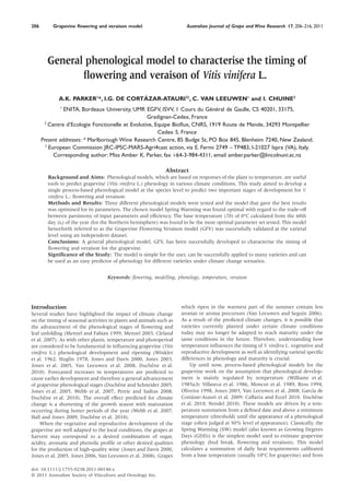
8. (a) Cabernet franc
Observation (DOY)
180 200 220 240 260 280
Prediction
(DOY)
180
200
220
240
260
280
(b) Cabernet-Sauvignon
Observation (DOY)
180 200 220 240 260 280
Prediction
(DOY)
180
200
220
240
260
280
(c) Chardonnay
Observation (DOY)
180 200 220 240 260 280
Prediction
(DOY)
180
200
220
240
260
280
(d) Chasselas
Observation (DOY)
180 200 220 240 260 280
Prediction
(DOY)
180
200
220
240
260
280
(e) Grenache
Observation (DOY)
180 200 220 240 260 280
Prediction
(DOY)
180
200
220
240
260
280
(f) Merlot
Observation (DOY)
180 200 220 240 260 280
Prediction
(DOY)
180
200
220
240
260
280
(g) Pinot noir
Observation (DOY)
180 200 220 240 260 280
Prediction
(DOY)
180
200
220
240
260
280
(h) Riesling
Observation (DOY)
180 200 220 240 260 280
Prediction
(DOY)
180
200
220
240
260
280
(i) Sauvignon blanc
Observation (DOY)
180 200 220 240 260 280
Prediction
(DOY)
180
200
220
240
260
280
(j) Syrah
Observation (DOY)
180 200 220 240 260 280
Prediction
(DOY)
180
200
220
240
260
280
(k) Ugni blanc
Observation (DOY)
180 200 220 240 260 280
Prediction
(DOY)
180
200
220
240
260
280
Figure 5. Observed and
simulated dates of veraison of
11 varieties using the Grapevine
Flowering Veraison model.
Closed circles (䊉) represent
data used for the model
parameterisation; open circles
(䊊) represent data used for the
model validation.
Parker et al. Grapevine flowering and veraison model 213
© 2011 Australian Society of Viticulture and Oenology Inc.

9. Heat requirements at the varietal level: model application
Using the phenological records, we parameterised the GVF
model for a large number of varieties (43 varieties for flowering
and 45 varieties for veraison corresponding to a total of 1092
and 980 observations, respectively) and the model successfully
predicted flowering and veraison for 11 varieties using an inde-
pendent dataset (440 flowering observations and 424 veraison
observations). For both phenological stages, the average quality
of prediction by variety (RMSE) was in most cases less than
1 week. The model validation indicated that the model can be
very efficient at the variety level, but the predictive power was
not necessarily equivalent for all varieties and both phenological
stages. The data used for parameterisation and validation corre-
spond to 55 and 67% of all the data collected in the study
(Table 1) for flowering and veraison, respectively. Further work
will be necessary to refine the F* values for each variety by
combining all records available as presented in the complete
dataset summarised in Table 1. However, for the 11 varieties
used in the validation process, the initial estimates of F* should
not change substantially given the similarity of results obtained
for model selection and validation.
It is possible that varieties may differ in their rate of devel-
opment between stages and their sensitivity to a given tempera-
ture may change as a function of this rate (Pouget 1966,
Buttrose 1969, Moncur et al. 1989, Calo et al. 1994). One limi-
tation of the type of model approach presented is that varieties
Table 6. Statistical analysis of the Grapevine Flowering Veraison model parameterised for flowering for the 11
varieties used for the validation process.
Variety F* n EF RMSE
Model
parameterisation
Model
validation
Model
parameterisation
Model
validation
Model
parameterisation
Model
validation
Cabernet franc 1225 57 45 0.73 0.53 5.13 5.45
Cabernet-Sauvignon 1270 70 62 0.83 0.46 3.46 3.65
Chardonnay 1217 100 71 0.78 0.73 5.15 4.69
Chasselas 1274 59 9 0.79 0.31 6.67 3.91
Grenache 1269 92 49 0.78 0.79 4.90 2.75
Merlot 1266 83 24 0.78 0.77 4.24 1.75
Pinot noir 1219 122 29 0.76 0.66 5.50 4.19
Riesling 1242 47 9 0.76 0.45 3.37 0.86
Sauvignon blanc 1238 37 57 0.77 0.63 2.72 3.27
Syrah 1277 92 35 0.84 0.77 3.68 2.33
Ugni blanc 1376 45 50 0.85 0.54 2.81 2.72
F* is the critical degree-day sum (above 0°C) fitted for each variety that was estimated from the model parameterisation dataset. n is the number observations by
variety used for the model choice and validation process. EF is the efficiency of the model; RMSE is the root means squared error in days.
Table 7. Statistical analysis of the Grapevine Flowering Veraison model parameterised for veraison for 11 varieties
used for the validation process.
Variety F* n EF RMSE
Model
parameterisation
Model
validation
Model
parameterisation
Model
validation
Model
parameterisation
Model
validation
Cabernet franc 2655 57 22 0.62 0.06 6.54 9.79
Cabernet-Sauvignon 2641 66 105 0.83 0.27 5.75 8.03
Chardonnay 2541 54 48 0.86 0.62 6.65 6.32
Chasselas 2342 53 9 0.88 -0.26 6.11 6.04
Grenache 2750 80 36 0.90 0.76 5.67 7.56
Merlot 2627 90 71 0.79 0.62 6.49 6.44
Pinot noir 2507 70 10 0.78 -1.82 7.81 8.07
Riesling 2584 43 9 0.77 0.27 7.06 4.48
Sauvignon blanc 2517 29 33 0.82 0.74 6.17 5.13
Syrah 2598 78 32 0.90 0.84 5.19 6.19
Ugni blanc 2777 41 49 0.90 -0.10 6.32 9.05
F* is the critical degree-day sum (above 0°C) fitted for each variety that was estimated from the model parameterisation dataset. n is the number observations by
variety used for the model choice and validation process. EF is the efficiency of the model; RMSE is the root means squared error in days.
214 Grapevine flowering and veraison model Australian Journal of Grape and Wine Research 17, 206–216, 2011
© 2011 Australian Society of Viticulture and Oenology Inc.

10. will invariably be at different stages during the developmental
cycle when the thermal summation begins and their individual
rate of development and temperature sensitivity would not be
accounted for. Some recent work has considered adapting more
complex models to specific varieties (Caffarra and Eccel 2010)
and this is an area of research that needs more investigation.
However, the GFV model remains advantageous for (i) under-
standing differences in phenological timing for a wide range of
varieties compared within the same modelling framework, (ii)
when considering rare or less data-rich varieties for which a
separate model may be difficult to achieve, and (iii) its simplicity
for the user. Given that the data used were spatially and tem-
porally diverse, corresponding to a wide range of varieties, the
current database can be used to explore the GFV model on the
varietal level in the future.
Model implications in a context of climate change
Climate change is predicted to advance phenology and ripening;
this can be countered to some extent by later ripening clones
and some viticultural practices such as late pruning (Friend and
Trought 2007 and references within). However, another possi-
bility is to consider changing to different varieties, which could
potentially develop and ripen later in the season. This paper has
taken the first steps towards successfully predicting flowering
and veraison for a range of varieties using one model that
in application will help identify suitable varieties for selected
climates.
Phenological modelling with climate change scenarios can
be used to predict the distribution of varieties in the future (see
Duchêne et al. 2010; Garcia de Cortazar-Atauri et al. 2010). The
current model was calibrated using a database containing a
diverse range of varieties; therefore, this model can be used to
better characterise heat requirements of a wide range of variet-
ies and of varieties for which little information is known thus
far. In combination with an understanding of future climate
change scenarios, such information will allow viticulturists to
have a better understanding of which varieties may better
perform in future temperature regimes, and direct them in
selection of alternate varieties.
Conclusion
We have shown that general process-based models can be
successfully applied and validated for the grapevine. A simple
model, GFV, corresponding to SW (t0 at 60 days, Tb value of 0°C)
has been selected, optimised and shown to be efficient to predict
flowering and veraison at the species and varietal level. The
model was validated and had greater predictive power than
existing models. Its simplicity makes it easy to use, and enables
further adoption of the model to predict the varietal timing of
flowering and veraison under a changing climate.
Acknowledgements
We acknowledge all research institutes, extension services and
private companies that willingly contributed to the collection of
phenological data. We are especially grateful to the following
people and their associated institutions for their generous con-
tributions to the database: B. Baculat (PHENOCLIM), M. Badier
(Chambre Agriculture 41), G. Barbeau (INRA-Angers), B. Bois
(Université de Bourgogne), J.-M. Boursiquot (Domaine de
Vassal), J.-Y. Cahurel (Institut Français de la Vigne et du Vin),
M. Claverie (Institut Français de la Vigne et du Vin), B. Daulny
(SICAVAC),T. Dufourcq (Institut Français de la Vigne et du
Vin), G. Guimberteau (INRA Bordeaux), O. Jacquet (Chambre
d’Agriculture de Vaucluse), S. Koundouras, T. Lacombe
(Domaine de Vassal), C. Lecareux (Chambre Agriculture 11), A.
Mançois (Lycée Ambois), C. Monamy (BIVB), H. Ojeda (INRA-
Pech Rouge), L. Panagai (CIVC), J.-C. Payan (Institut Français
de la Vigne et du Vin), B. Rodriguez (Syndicat Général des
Vignerons des Côtes du Rhône), I. Sivadon (CIRAME), J.-P.
Soyer (INRA Bordeaux), J.-L. Spring (Agroscope Pully), C.
Schneider (INRA Colmar), G. Silva (CIVAM) P. Storchi (CRA-
VIC), D. Tomasi (CRA – VIT) and W. Trambouze (Chambre
Agriculture 34).
References
Bidabe, B. (1965a) Contrôle de l’époque de floraison du pommier par une
nouvelle conception de l’action des températures. Comptes rendus des
Séances de l’Académie d’Agriculture de France 49, 934–945.
Bidabe, B. (1965b) L’action des températures sur l’évolution des bourgeons
de l’entrée en dormance à la floraison. 96th Congrès Pomologique, France
(Société Pomologique de France: France) pp. 51–56.
Burnham, K.P. and Anderson, D.R. (2002) Model selection and multimodel
inference: a practical information-theoretic approach (Springer-Verlag:
New York).
Buttrose, M.S. (1969) Vegetative growth of grapevine varieties under con-
trolled temperature and light intensity. Vitis 8, 280–285.
Caffarra, A. and Eccel, E. (2010) Increasing robustness of phenological
models for Vitis vinifera cv. Chardonnay. International Journal of Bio-
meteorology 54, 255–267.
Calo, A., Tomasi, D., Costacurta, A., Biscaro, S. and Aldighieri, R. (1994)
The effect of temperature thresholds on grapevine (Vitis sp.) bloom: an
interpretative model. Rivista di Viticoltura e di Enologia 47, 3–14.
Cesaraccio, C., Spano, D., Snyder, R.L. and Duce, P. (2004) Chilling and
forcing model to predict bud-burst of crop and forest species. Agricultural
and Forest Meteorology 126, 1–13.
Chuine, I. (2000) A unified model for budburst of trees. Journal of Theo-
retical Biology 207, 337–347.
Chuine, I., Cour, P. and Rousseau, D.D. (1998) Fitting models predicting
dates of flowering of temperature-zone trees using simulated annealing.
Plant, Cell and Environment 21, 455–466.
Chuine, I., Kramer, K. and Hänninen, H. (2003) Plant development
models. In: Phenology: an integrative environmental science, 1st edn. Ed.
M.D. Schwartz (Kluwer Press: Milwaukee, WI) pp. 217–235.
Cleland, E., Chuine, I., Menzel, A., Mooney, H. and Schwartz, M. (2007)
Shifting plant phenology in response to global change. Trends in Ecology
and Evolution 22, 357–365.
Coombe, B.G. (1995) Adoption of a system for identifying grapevine growth
stages. Australian Journal of Grape and Wine Research 1, 104–110.
Crepinsek, Z., Kajfez-Bogataj, L. and Bergant, K. (2006) Modelling of
weather variability effect on fitophenology. Ecological Modelling 194,
256–265.
Duchêne, E. and Schneider, C. (2005) Grapevine and climatic changes: a
glance at the situation in Alsace. Agronomy for Sustainable Development
25, 93–99.
Duchêne, E., Huard, F., Dumas, V., Schneider, C. and Merdinoglu, D.
(2010) The challenge of adapting grapevine varieties to climate change.
Climate Research 41, 193–204.
Friend, A. and Trought, M.C.T. (2007) Delayed winter spur pruning can
alter yield components of Merlot grapevines. Australian Journal of Grape
and Wine Research 13, 157–164.
García de Cortázar-Atauri, I., Brisson, N. and Gaudilliere, J.-P. (2009)
Performance of several models for predicting budburst date of grapevine
(Vitis vinifera L.). International Journal of Biometeorology 53, 317–326.
Garcia de Cortazar-Atauri, I., Chuine, I., Donatelli, M., Parker, A.K. and
van Leeuwen, C. (2010) A curvilinear process-based phenological model
to study impacts of climate change on grapevine (Vitis vinifera L.). Pro-
ceedings of Agro 2010: the 11th ESA Congress, Montpellier, France
(Agropolis International Editions: Montpellier) pp. 907–908.
Gladstones, J. (1992) Viticulture and environment (Winetitles: Adelaide).
Greenwood, D.J., Neeteson, J.J. and Draycott, A. (1985) Response of
potatoes to N fertilizer: dynamic model. Plant Soil 85, 185–203.
Hall, A. and Jones, G.V. (2009) Effect of potential atmospheric warming on
temperature-based indices describing Australian winegrape growing con-
ditions. Australian Journal of Grape and Wine Research 15, 97–119.
Huglin, P. (1978) Nouveau mode d’évaluation des possibilités héliother-
miques d’un milieu viticole. Comptes rendus des Séances de l’Académie
d’Agriculture de France 64, 1117–1126.
Jones, G. (2006) Climate change and wine: observations, impacts and
future implications. Wine Industry Journal 21, 21–26.
Parker et al. Grapevine flowering and veraison model 215
© 2011 Australian Society of Viticulture and Oenology Inc.

11. Jones, G.V. (2003) Winegrape phenology. In: Phenology: an integrative
environmental science, 1st edn. Ed. M.D. Schwartz (Kluwer Press: Mil-
waukee, MA) pp. 523–539.
Jones, G.V. and Davis, R.E. (2000) Climate influences on grapevine phe-
nology, grape composition, and wine production and quality for Bor-
deaux, France. American Journal of Enology and Viticulture 51, 249–261.
Jones, G.V., White, M.A., Cooper, O.R. and Storchmann, K. (2005)
Climate change and global wine quality. Climatic Change 73, 319–343.
Menzel, A. (2003) Plant phenological anomalies in Germany and their
relation to air temperature and NAO. Climatic Change 57, 243–263.
Menzel, A. and Fabian, P. (1999) Growing season extended in Europe.
Nature 397, 659.
Moncur, M.W., Rattigan, K., MacKenzie, D.H. and McIntyre, G.N. (1989)
Base temperatures for budbreak and leaf appearance of grapevines.
American Journal of Enology and Viticulture 40, 21–26.
Nendel, C. (2010) Grapevine bud break prediction for cool winter climates.
International Journal of Biometeorology 54, 231–241.
Oliveira, M. (1998) Calculation of budbreak and flowering base tempera-
tures for Vitis vinifera cv. Touriga Francesa in the Duoro Region of Portugal.
American Journal of Enology and Viticulture 49, 74–78.
Petrie, P.R. and Sadras, V.O. (2008) Advancement of grapevine maturity in
Australia between 1993 and 2006: putative causes, magnitude of trends
and viticultural consequences. Australian Journal of Grape and Wine
Research 14, 33–45.
Pouget, R. (1966) Etude du Rythme végétatif: caractères physiologiques lié
a la précocité de débourrement chez la vigne. Annales de l’Amelioriation
des Plantes 16, 81–100.
Riou, C. (1994) The effect of climate on grape ripening: application to the
zoning of sugar content in the European community (European Commis-
sion: Luxembourg) p. 319.
Van Leeuwen, C. and Seguin, G. (2006) The concept of terroir in viticul-
ture. Journal of Wine Research 17, 1–10.
Van Leeuwen, C., Garnier, C., Agut, C., Baculat, B., Barbeau, G., Besnard,
E., Bois, B., Boursiquot, J.-M., Chuine, I., Dessup, T., Dufourcq, T.,
Garcia-Cortazar, I., Marguerit, E., Monamy, C., Koundouras, S., Payan,
J.-C., Parker, A., Renouf, V., Rodriguez-Lovelle, B., Roby, J.-P., Tonietto,
J. and Trambouze, W. (2008) Heat requirements for grapevine varieties
are essential information to adapt plant material in a changing climate.
Proceedings of the 7th International Terroir Congress, Changins, Switzer-
land (Agroscope Changins-Wädenswil: Switzerland) pp. 222–227.
Villaseca, S.C., Novoa, R.S.-A. and Muñoz, I.H. (1986) Fenologia y sumas
de temperaturas en 24 variedades de vid. Agricultura Técnica Chile 46,
63–67.
Webb, L.B., Whetton, P.H. and Barlow, E.W.R. (2007) Modelled impact of
future climate change on the phenology of winegrapes in Australia. Aus-
tralian Journal of Grape and Wine Research 13, 165–175.
Williams, D.W., Williams, L.E., Barnett, W.W., Kelley, K.M. and McKendry,
M.V. (1985a) Validation of a model for the growth and development of the
Thompson Seedless Grapevine. I. Vegetative growth and fruit yield.
American Journal of Enology and Viticulture 36, 275–282.
Williams, D.W., Andris, H.L., Beede, R.H., Luvisi, D.A., Norton, M.V.K. and
Williams, L.E. (1985b) Validation of a model for the growth and devel-
opment of the Thompson Seedless Grapevine. II. Phenology. American
Journal of Enology and Viticulture 36, 283–289.
Winkler, A.J., Cook, J.A., Kliewer, W.M. and Lider, L.A. (1962) General
viticulture (University of California Press: Berkeley and Los Angeles, CA).
Manuscript received: 15 October 2010
Revised manuscript received: 13 January 2011
Accepted: 1 February 2011
216 Grapevine flowering and veraison model Australian Journal of Grape and Wine Research 17, 206–216, 2011
© 2011 Australian Society of Viticulture and Oenology Inc.