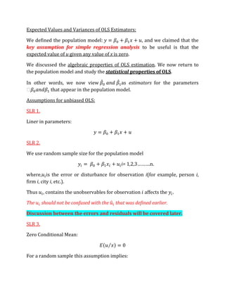
1. Expected Values and Variances of OLS Estimators:
We defined the population model , and we claimed that the
key assumption for simple regression analysis to be useful is that the
expected value of u given any value of x is zero.
We discussed the algebraic properties of OLS estimation. We now return to
the population model and study the statistical properties of OLS.
In other words, we now view as estimators for the parameters
��� that appear in the population model.
Assumptions for unbiased OLS:
SLR 1.
Liner in parameters:
SLR 2.
We use random sample size for the population model
i= 1,2,3……….n.
where, is the error or disturbance for observation i(for example, person i,
firm i, city i, etc.).
Thus , contains the unobservables for observation affects the .
The should not be confused with the that was defined earlier.
Discussion between the errors and residuals will be covered later.
SLR 3.
Zero Conditional Mean:
For a random sample this assumption implies:

2. SLR 4.
The sample variation in the independent variable:
This means if = wage and = education then SLR. 4 fail only if every one in
the sample has the same amount of education. This is hardly true!
USING SLR1.- SLR4,
for any values of In other words are unbiased estimates for
Variance in OLS estimators:
Once we know that are unbiased estimates for we must also
know how far do we expect to be from on an average.
Among other things this allows us to choose the best estimator among all, or at
least a broad class of unbiased estimators.
SLR 5.
This is the homoskedasity Assumption.
This assumption plays no role in showing are unbiased estimators
of���
is often called the error variance or disturbance variance.

3. ** Note
Under Assumption SLR.1 through SLR.5
Where these are conditional on the sample values
Note: All the quantities of entering in the preceding equations except can
be estimated from the data.

4. But variance can be estimated using the following formula (IF YOU WANT
REFER TO APPENDIX 3.A)
Estimating the Error in Variance:
So far we know that:
And
.
Difference between errors (or disturbance)and residuals is crucial for
constructing .
Population model in terms of randomly observed sample can be written as:
and is the ERROR for observation
in terms of fitted value can be expressed as:
and is the RESIDUAL for observation
Thus:
We saw previously that for OLS to be unbiased .
But .
The difference between them does not have a zero expected value.
Now returning to :

5. Thus the unbiased “estimator” for is:
But since we do not observer and observe only the OLS residual of
.
This is the true estimator, because it gives a complete rule for any sample data
on on
One slight drawback to this estimator is that it turns out to be biased
(although for large the bias is small).
The is biased only because it does not account for two restrictions that
OLS satisfies:
Since there are only n-2 degrees of freedom in OLS residuals (as opposed to
degrees of freedom in errors)
If we apply the restrictions in are replace with the above restrictions
would no longer hold.
The unbiased estimator of we will use makes degrees-of-freedom
adjustment:
*This estimator is also denoted as
Properties of OLS Estimators:
If assumption 1 through 4 hold then the estimators determined by
OLS are known as Best Liner Unbiased Estimates (BLUE).
What does BLUE stand for?

6. "Estimator" - is an estimator of true value of .
"Linear"- is linear in parameter.
"Unbiased" – On average, the actual value of the will represent the
true values.
"Best" – Means of OLS estimator has minimum variance among the class of
linear unbiased estimators. The Gauss – Markov theorem provides of that of
OLS estimator is best.
**Note