Exploring DEM error with geographically weighted regression
•
2 gostaram•473 visualizações

Michal Gallay, Christopher D. Lloyd, Jennifer McKinley: Exploring DEM error with geographically weighted regression (poster), 9th International Symposium GIS Ostrava, VŠB – Technical Univerzity of Ostrava, from 23rd to 25th January 2012
Recomendados

Recomendados
Mais conteúdo relacionado
Mais procurados
Mais procurados (20)
Destaque
Destaque (8)
Semelhante a Exploring DEM error with geographically weighted regression
Semelhante a Exploring DEM error with geographically weighted regression (20)
Mais de GeoCommunity
Mais de GeoCommunity (8)
Último
Último (20)
Exploring DEM error with geographically weighted regression
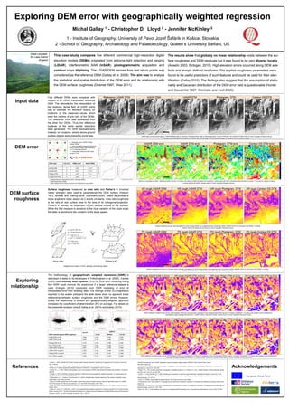
- 1. Exploring DEM error with geographically weighted regression Michal Gallay 1 - Christopher D. Lloyd 2 - Jennifer McKinley 2 1 - Institute of Geography, University of Pavol Jozef Šafárik in Košice, Slovakia 2 - School of Geography, Archaeology and Palaeoecology, Queen’s University Belfast, UK Area ratio Fisher’s K Adapted from Hobson (1972), McKean and Roering (2004) Input data DEM error DEM surface roughness Exploring relationship 0.6680.4560.1840.001InSAR DSM vs log(FK) 0.6380.4050.2020.002InSAR DTM vs log(FK) 0.6650.4270.2010.001Photog.DTM vs log(FK) 0.6830.4190.1870.033Cont. DTM vs log(FK) 0.7110.4660.2340.014Cont. DTM vs AR 0.6920.4660.2350.016Photog.DTM vs AR 0.6420.4020.1850.030InSAR DTM vs AR 0.6760.4970.2730.024InSAR DSM vs AR 3rd QrtMedian1st Qrt GWR R2 OLS R2 DEM residuals against DEM roughness * unobstructed and obstructed flat land, Intermap (2002), ** GeoPerspectives (2006), *** with respect to the contour interval 10 m Ordnance Survey (2001) 5 ***3.045Contour OS DTM 1.5 **2.765Photog. DTM 1 , 2.5 *3.675InSAR DTM 1 , 2.5 *3.665InSAR DSM Units in metres Stated RMSERMSE maskCell sizeDEM origin The methodology of geographically weighted regression (GWR) is described in detail by its developers in Fotheringham et al. (2002). Carlisle (2005) used ordinary least squares (OLS) for DEM error modelling noting that GWR could improve the predictions if a larger reference dataset is used. Erdogan (2010) conducted such GWR modelling of error of interpolated DEM from levelling data. The findings of the OLS regression reported in the scatter plots and the table below show no apparent linear relationship between surface roughness and the DEM errors. However, locally the relationship is evident and geographically weighted approach increases the cooefficient of determination (R2) on average. For details on the presented analysis consult Gallay et al. (2010) and Gallay (2010). This case study compares five different commercial high-resolution digital elevation models (DEMs) originated from airborne light detection and ranging (LiDAR), interferometric SAR (InSAR), photogrammetric acquisition and contour maps digitizing. The LiDAR DEM derived from last return points was considered as the reference DEM (Gallay et al. 2008). The aim was to analyse the statistical and spatial distribution of the DEM error and its relationship with the DEM surface roughness (Desmet 1997, Wise 2011). ■ – observed value, InSAR, Photog., Contour DEMs ● – more accurately measured reference value LiDAR last return point elevations (ca. 2 m sampling interval) O – interpolated reference DEM value, cell size = 5 m Z■ – ZO = DEM error Surface roughness measured as area ratio and Fisher’s K (inverted vector strength) were used to parameterise the DEM surface (Hobson 1972, Mckean and Roering 2004, Grohmann 2004). Useful as proxies of slope angle and slope aspect as it avoids circularity. Area ratio roughness is the ratio of real surface area to the area of its orthogonal projection. Fisher’s K defines the dispersion of unit vectors normal to the surface. While the first measure is sensitive to the local variation of the slope angle the latter is sensitive to the variation of the slope aspect. The results show that globally no linear relationship exists between the sur- face roughness and DEM residuals but it was found to be very diverse locally (Anselin 2003, Erdogan, 2010). High elevation errors occurred along DEM arte- facts and sharply defined landforms. The applied roughness parameters were found to be useful predictors of such features and could be used for their iden- tification (Gallay 2010). The findings also suggest that the assumption of statio- narity and Gaussian distribution of the DEM error field is questionable (Hunter and Goodchild 1997, Wechsler and Kroll 2006). Great Langdale the Lake District England LiDAR data (c) Environment Agency, InSAR NextMap data (c) Intermap, Photogrammetric data (c) GeoPerspectives, Contour DTM data: OS LandForm Profile DTM (c) Crown Copyright Ordnance Survey. Shaded relief calculated in LandSerf (c) Jo Wood, sun azimuth angle 134°, sun elevation angle 10°, resoluti on of the DEMs 5 metres. DEM error calculated as ‘DEM – Reference DEM‘, cell size = 5 metres, the reference DEM calculated from last return LiDAR points with IDW in Geostat.Analyst ArcGIS 9.0, points = 12, power=2, cell size 5 metres. Contour interval 20 metres, contour lines (c) Crown Copyright Ordnance Survey. Surface roughness as area ratio calculated for a 5x5 moving window by r.roughness.vector (Grohmann 2004), GRASS GIS 6.2.2, cell sizes of the DEMs = 5 metres Contour interval 20 metres, contour lines (c) Crown Copyright Ordnance Survey. Surface roughness as Fisher’s K (inverted vector strength) calculated for a 5x5 moving window by r.roughness.vector (Grohmann 2004), GRASS GIS 6.2.2, cell sizes of the DEMs = 5 metres Contour interval 20 metres, contour lines (c) Crown Copyright Ordnance Survey. GWR coefficient of determination (R.sq). GWR between DEM error and area ratio roughness of the corresponding DEMs cell-size = 5 metres, bandwidth = 15 metres, gwr.weights: exp(-0.5(dist/bw)^2). Calculated by spgwr package (Bivand and Yu, 2008). Contour interval 20 metres, contour lines (c) Crown Copyright Ordnance Survey. GWR coefficient of determination (R.sq). GWR between DEM error and logarithm of Fisher’s K roughness of the corresponding DEMs cell-size = 5 metres, bandwidth = 15 metres, gwr.weights: exp(-0.5(dist/bw)^2). Calculated by spgwr package (Bivand and Yu, 2008). Contour interval 20 metres, contour lines (c) Crown Copyright Ordnance Survey. Four different DEMs were compared with respect to an LiDAR interpolated reference DEM. The rationale for the interpolation of the relatively dense field of LiDAR points was to estimate the elevation exactly on locations of the observed values which were the centres of grid cells of the DEMs. The reference DEM was subtracted from the other four DEMs. Thus, the difference surfaces of the same spatial resolution were generated. The DEM residuals were masked on locations where above-ground surface objects were present to avoid bias. References Acknowledgements European Social Fund • Anselin, L. (2003). GeoDa TM 0.9 User's Guide. Spatial Analysis Laboratory. Department of Agricultural and Consumer Economics. Univ. of Illinois. •Bivand, R. and Yu, D. (2008). spgwr: Geographically weighted regression. R package. version 0.5-4. •Carlisle, B. H. (2005), Modelling the Spatial Distribution of DEM Error. Transactions in GIS, 9: 521–540 • Desmet, P. J. J. (1997). Effects of interpolation errors on the analysis of DEMs. Earth Surface Processes and Landforms. Volume 22, 563-580. • Erdogan, S. (2010). Modelling the spatial distribution of DEM error with geographically weighted regression: An experimental study. Computers & Geosciences. Volume 36, 34-43. • Fotheringham, A. S., Charlton, M. and Brunsdon, C. (2002). Geographically weighted regression: The analysis of spatially varying relationships. John Wiley and Sons. • Gallay, M. (2008). Assessment of DTM quality: a case study using fine spatial resolution data from alternative sources In: GISRUK 2008: GIS research UK 16th annual conference : 2.-4. April 2008. Manchester, 2008. 156 p. • Gallay, M. (2010): Assessing alternative methods of acquiring and processing digital elevation data. PhD thesis. Queen's University Belfast. 339 p. • Gallay, M., Lloyd, C. D., McKinley, J. (2010): Using geographically weighted regression for analysing elevation error of high-resolution DEMs. Accuracy 2010 - The Ninth International Symposium on Spatial Accuracy Assessment in Natural Resources and Environmental Sciences, July 20 – 23, 2010. University of Leicester, UK, p. 109-112. •GRASS Development Team (2008). Geographic resources analysis support system (GRASS), GNU General Public License. http://grass.osgeo.org. • Grohmann, C. H. (2004). Morphometric analysis in geographic information systems: applications of free software GRASS and R. Computers & Geosciences. Volume 30, 1055-1067. • Hobson, R.D., 1972. Surface roughness in topography: quantitative approach. In: Chorley, R.J. (Ed.)., Spatial Analysis in Geomorphology. Harper and Row, New York, NY, pp. 225–245. • Hunter, G. J. and Goodchild, M. F. (1997). Modeling the uncertainty of slope and aspect estimates. Geographical Analysis. Volume 29, 35-49. • McKean, J. and Roering, J. (2004). Objective landslide detection and surface morphology mapping using high-resolution airborne laser altimetry. Geomorphology,, 57: 331-351. • Lloyd, C. D. (2006). Local models for spatial analysis. CRC/Taylor & Francis, Boca Raton. • R Development Core Team (2008).R: A language and environment for statistical computing. R Foundation for Statistical Computing. http://www.R- project.org. • Wechsler, S. P. and Kroll, C., N. (2006). Quantifying DEM uncertainty and its effect on topographic parameters. Photogrammetric Engineering and Remote Sensing, Volume 72, 1081-1090. • Wise, S.M. (2011). Cross-validation as a means of investigating DEM interpolation error. Computers and Geosciences, Volume 37(8), 978–991. O O OOO O O O O