Spit, Duct Tape, Baling Wire & Oral Tradition: Dealing With Radio Data
•
2 likes•834 views

Review talk by Prof. Oleg Smirnov at the SuperJEDI Conference, July 2013

Recommended
Recommended
More Related Content
Similar to Spit, Duct Tape, Baling Wire & Oral Tradition: Dealing With Radio Data
Similar to Spit, Duct Tape, Baling Wire & Oral Tradition: Dealing With Radio Data (20)
More from CosmoAIMS Bassett
More from CosmoAIMS Bassett (20)
Recently uploaded
Recently uploaded (20)
Spit, Duct Tape, Baling Wire & Oral Tradition: Dealing With Radio Data
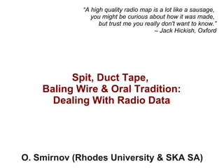
- 1. Spit, Duct Tape, Baling Wire & Oral Tradition: Dealing With Radio Data O. Smirnov (Rhodes University & SKA SA) “A high quality radio map is a lot like a sausage, you might be curious about how it was made, but trust me you really don't want to know.” – Jack Hickish, Oxford
- 2. O. Smirnov - SKA Challenges - SuperJEDI , Mauritius, Jul 2013 2 Radio Interferometer... What lay people think I do What funding agencies think I do What cosmologists & astrophysicists think I do What my engineers think I do What I actually do (In celebration of the passing of an extremely lame but blissfully short-lived internet meme)
- 3. O. Smirnov - SKA Challenges - SuperJEDI , Mauritius, Jul 2013 3 The Ron Ekers Seven-Step Program To Producing A Radio Interferometer Step 0. Admit that you have a problem: You want to (need to/are forced to by peers/supervisors) to do interferometry. “My name is Oleg Smirnov, and I am an interferometrist.”
- 4. O. Smirnov - SKA Challenges - SuperJEDI , Mauritius, Jul 2013 4 How To Make An Interferometer 1 Start with a normal reflector telescope....
- 5. O. Smirnov - SKA Challenges - SuperJEDI , Mauritius, Jul 2013 5 How To Make An Interferometer 2 Then break it up into sections...
- 6. O. Smirnov - SKA Challenges - SuperJEDI , Mauritius, Jul 2013 6 How To Make An Interferometer 3 Replace the optical path with electronics
- 7. O. Smirnov - SKA Challenges - SuperJEDI , Mauritius, Jul 2013 7 How To Make An Interferometer 4 Move the electronics outside the dish ...and add cable delays
- 8. O. Smirnov - SKA Challenges - SuperJEDI , Mauritius, Jul 2013 8 How To Make An Interferometer 5 Why not drop the pieces onto the ground?
- 9. O. Smirnov - SKA Challenges - SuperJEDI , Mauritius, Jul 2013 9 How To Make An Interferometer 6 ...all of them
- 10. O. Smirnov - SKA Challenges - SuperJEDI , Mauritius, Jul 2013 10 How To Make An Interferometer 7 And now replace them with proper radio dishes. ...and that's all! (?) Well almost, what about the other pixels?
- 11. O. Smirnov - SKA Challenges - SuperJEDI , Mauritius, Jul 2013 11 How Does Optical Imaging Do It? This bit sees the EMF from all directions, added up together. This bit sees the EMF from all parts of the dish surface, added up together. ∬S l ,me iulvm dl dm
- 12. O. Smirnov - SKA Challenges - SuperJEDI , Mauritius, Jul 2013 12 Fourier Transforms An optical imaging system implicitly performs two Fourier transforms: 1. Aperture EMF distribution = FT of the sky 2. Focal plane = FT-1 of the aperture EMF A radio interferometer array measures (1) Then we do the second FT in software Hence, “aperture synthesis” imaging
- 13. O. Smirnov - SKA Challenges - SuperJEDI , Mauritius, Jul 2013 13 The uv-Plane FT Image plane uv-plane (12 hours!) In a sense, the two are entirely equivalent One baseline samples one visibility at a time
- 14. O. Smirnov - SKA Challenges - SuperJEDI , Mauritius, Jul 2013 14 Earth Rotation Aperture Synthesis Every pair of antennas (baseline) is correlated, measures one complex visibility = one point on the uv-plane. As the Earth rotates, a baseline sweeps out an arc in the uv-plane See uv-coverage plot (previous slide) Even a one-dimensional East-West array (WSRT = 14 antennas) is sufficient
- 15. O. Smirnov - SKA Challenges - SuperJEDI , Mauritius, Jul 2013 15 Where's The Catch? We don't measure the full uv-plane, thus we can never recover the image fully (missing information) Interferometer = high & low-pass filter Every visibility measurement is distorted (complex receiver gains, etc.), needs to be calibrated. (Doesn't work the same way in optical interferometry at all...) Can't really form up complex visibilities, etc.
- 16. O. Smirnov - SKA Challenges - SuperJEDI , Mauritius, Jul 2013 16 Catch 1: Missing Information Response to a point source: Point Spread Function (PSF) PSF = FT(uv-coverage) Observed “dirty image” is convolved with the PSF Structure in the PSF = uncertainty in the flux distribution (corresponding to missing data in the uv-plane) (12-hour WSRT PSF) 24
- 17. O. Smirnov - SKA Challenges - SuperJEDI , Mauritius, Jul 2013 17 Deconvolution: from dirty to clean images A whole continuum of skies fits the dirty image (pick any value for the missing uv-components) Deconvolution picks one = interpolates the missing info from extra assumptions (e.g.: “sources are point-like”). Real-life WSRT dirty image Dirty image dominated by PSF sidelobes from the stronger sources Deconvolution required to get at the faint stuff underneath.
- 18. O. Smirnov - SKA Challenges - SuperJEDI , Mauritius, Jul 2013 18 Deconvolution Gone Bad Extended sources always troublesome Plus we're missing the zero- order spacing measurement (=total power) ...end up with a “negative bowl” problem Ultimately, interpolating missing uv-components requires a better choice of basis functions ...and better deconvolution methods Compressive sensing (CS) is promising
- 19. O. Smirnov - SKA Challenges - SuperJEDI , Mauritius, Jul 2013 19 Catch 2: Measurement Errors Incoming signal is subject to distortions (refraction, delay, amplitude loss) atmospheric and electronic
- 20. O. Smirnov - SKA Challenges - SuperJEDI , Mauritius, Jul 2013 20 An Uncalibrated Interferometer Complex gain error: signal multiplied by a amplitude and phase delay term Delay errors correspond to differences in arrival time, i.e. random shifts of antennas towards and away from the source Amplitude errors = different sensitivities
- 21. O. Smirnov - SKA Challenges - SuperJEDI , Mauritius, Jul 2013 21 ...And Its Optical Equivalent
- 22. O. Smirnov - SKA Challenges - SuperJEDI , Mauritius, Jul 2013 22 And The Result... One point-like source, but observed with phase errors In the uv-plane, phase encodes information about location Phase errors tend to spread the flux around Amplitude errors distort structure And Dr Sidelobes ensures that the damage is distributed democratically
- 23. O. Smirnov - SKA Challenges - SuperJEDI , Mauritius, Jul 2013 23 Stone-Age Calibration (First-Generation, or 1GC) Calibrate gains using a known calibrator source Move antennas to target, cross your fingers, and hope that everything stays stable enough to get an image Dynamic range: ~100:1 V pq=g pq M pq Gain of interferometer (i.e. antenna pair) p-q Model visibility Observed visibility
- 24. O. Smirnov - SKA Challenges - SuperJEDI , Mauritius, Jul 2013 24 The Selfcal Revolution (2GC) Per-baseline gains are actually products of per- antenna complex gains! Vpq : observed visibility Mpq : model visibility (FT of sky) gp : antenna p complex gain N(N-1)/2 visibilities >> N gains Start with simple M Solve for g's Improve M, rinse & repeat dynamic range > 106 :1 V pq=g p ̄gq M pq
- 25. O. Smirnov - SKA Challenges - SuperJEDI , Mauritius, Jul 2013 25 Typical Selfcal Cycle Pre-calibrate g using external calibrators Correct with g-1 , make dirty image, deconvolve Generate rough initial sky model Solve for g using the current sky model Correct with g-1 , make dirty image, deconvolve Optional: subtract model and work with residuals Update the sky model pre-calSelfcalloop Huge body of experience suggests that this works rather well, BUT there's no formal proof (!!!) Current practice is a collection of ad hoc methods, dark art and lore passed down the generations in what is virtually an oral tradition.
- 26. O. Smirnov - SKA Challenges - SuperJEDI , Mauritius, Jul 2013 26 The Essense Of Selfcal Essentially, selfcal is model fitting: Sky model (image of the sky): M(x,y,υ) Instrument model (set of gains): {gp (υ,t)} Fit this to the observed data With alternating updates of M and g
- 27. O. Smirnov - SKA Challenges - SuperJEDI , Mauritius, Jul 2013 27 Fundamental Assumption Basic assumption of selfcal: every antenna sees the same (constant) sky, but has its own (time-variable) complex gain term. V pq=g p gq M pq
- 28. O. Smirnov - SKA Challenges - SuperJEDI , Mauritius, Jul 2013 28 The Past: Massive Overengineering (Built For 1GC, used with 2GC)
- 29. O. Smirnov - SKA Challenges - SuperJEDI , Mauritius, Jul 2013 29 The Future: Four Sticks In The Ground (+Software)
- 30. O. Smirnov - SKA Challenges - SuperJEDI , Mauritius, Jul 2013 30 ...and Dishes Made Of Plastic (+Compatible Software)
- 31. O. Smirnov - SKA Challenges - SuperJEDI , Mauritius, Jul 2013 31
- 32. O. Smirnov - SKA Challenges - SuperJEDI , Mauritius, Jul 2013 32 Catch 3: Direction Dependence Distortions on incoming signal depend on time, antenna and direction Esp. with wide field/low frequency/high sensitivity Fortunately, have a formalism to describe this: the RIME (Radio Interferometer Measurement Equation)
- 33. O. Smirnov - Problems of Radio Interferometric Data Reduction - FASTAR/Espresso Workshop - 30/10/2012 33 The Basics: Vectors & Jones Matrices e= ex ey v=J e= j11 j12 j21 j22 ex ey A dual-receptor feed measures two complex voltages (polarizations): A transverse EM field can be described by a complex vector: v= vx vy We assume all propagation effects are linear. Any linear transform of a vector can be described by a matrix: x y z
- 34. O. Smirnov - Problems of Radio Interferometric Data Reduction - FASTAR/Espresso Workshop - 30/10/2012 34 Correlation e vp=J p e vq=Jq e vxx=〈vpx vqx * 〉 vyy=〈vpy vqy * 〉 vxy=〈vpx vqy * 〉 vyx=〈vpy vqx * 〉 The same signal reaches antennas p and q along two different paths. We then correlate the two sets of complex voltages.
- 35. O. Smirnov - Problems of Radio Interferometric Data Reduction - FASTAR/Espresso Workshop - 30/10/2012 35 The 2×2 Visibility Matrix An interferometer correlates the vectors vp ,vq : vxx=〈vpx vqx * 〉,vxy=〈vpx vqy * 〉 ,vyx=〈vpy vqx * 〉,vyy=〈vpy vqy * 〉 Let us write this as a matrix product: V pq=2〈vp vq † 〉=2〈 vpx vpy vqx * vqy * 〉=2 vxx vxy vyx vyy (〈 〉: time/freq averaging; † : conjugate-and-transpose) V pq is also called the visibility matrix.
- 36. O. Smirnov - Problems of Radio Interferometric Data Reduction - FASTAR/Espresso Workshop - 30/10/2012 36 Coherencies & Stokes Parameters Antennas p,q measure vp= Jp e , vq= Jq e. Therefore: Vpq=2〈 Jp e Jq e † 〉=2〈 Jpee † Jq † 〉= Jp2〈ee † 〉 Jq † (making use of AB † =B † A † , and assuming Jp is constant over 〈 〉) The inner quantity is called the coherency or brightness, and (by definition of the Stokes parameters) is actually: B=2〈ee † 〉≡ IQ UiV U−iV I−Q I≡〈∣ex∣2 〉〈∣ey∣2 〉=〈ex ex * 〉〈ey ey * 〉 , Q≡〈∣ex∣2 〉−〈∣ey∣2 〉=〈ex ex * 〉−〈ey ey * 〉 , etc.
- 37. O. Smirnov - Problems of Radio Interferometric Data Reduction - FASTAR/Espresso Workshop - 30/10/2012 37 And That's The RIME! XX XY YX YY = jxx p jxy p jyx p jyy p IQ UiV U−iV I−Q jxxq * jyxq * jxyq * jyyq * Vpq= Jp B Jq † The RIME, in its simplest form: measured antenna qantenna p source
- 38. O. Smirnov - Interferometry II & The Measurement Equation - October 2012 38 Accumulating Jones Matrices If Jp , Jq are products of Jones matrices: Jp= Jpn ... Jp1 , Jq= Jqm... Jq1 Since (AB)H =BH AH , the M.E. becomes: Vpq= Jpn ... Jp2 Jp1 B Jq1 H Jq2 H ... Jqm H or in the "onion form": Vpq= Jpn(...( Jp2( Jp1 B Jq1 H ) Jq2 H )...) Jqm H
- 39. O. Smirnov - Problems of Radio Interferometric Data Reduction - FASTAR/Espresso Workshop - 30/10/2012 39 The Classical (2GC) Approach To Polarization Calibration U V Q
- 40. O. Smirnov - Problems of Radio Interferometric Data Reduction - FASTAR/Espresso Workshop - 30/10/2012 40 RIME version: V pq=Gp Dp X Dq † Gq † Scalar Equations For Polarization Selfcal
- 41. O. Smirnov - SKA Challenges - SuperJEDI , Mauritius, Jul 2013 41 Off-Axis Effects 3C147 @21cm 12h WSRT synthesis 160 MHz bandwidth 22 Jy peak (3C147) 13.5 μJy noise 1,600,000:1 DR thermal noise-limited Regular calibration does not reach the noise, leaves off-axis artefacts due to direction-dependent effects (left inset) Addressed via differential gains (right inset) 3C147 22Jy 30 mJy
- 42. 26/07/11 O. Smirnov - Primary Beams, Pointing Errors & The Westerbork Wobble - CALIM2011, Manchester 42 Differential Gains, In a Nutshell Vpq= Gp gain & bandpass ∑ s dEp s differential gain Ep s beam Xpq source coherency Eq s† dEq s† sum over sources Gq † dEp s is frequency-independent, slowly varying in time. Solvable for a handful of "troublesome" sources, and set to unity for the rest.
- 43. O. Smirnov - SKA Challenges - SuperJEDI , Mauritius, Jul 2013 43 JVLA Version Recent result from 3GC3 workshop 3C147 JVLA-D @1.4 GHz Best image after regular selfcal
- 44. O. Smirnov - SKA Challenges - SuperJEDI , Mauritius, Jul 2013 44 JVLA Version Recent result from 3GC3 workshop 3C147 JVLA-D @1.4 GHz Best image after regular selfcal ...and direction- dependent (DD) calibration on a few sources
- 45. O. Smirnov - SKA Challenges - SuperJEDI , Mauritius, Jul 2013 45 KAT-7 Version
- 46. O. Smirnov - SKA Challenges - SuperJEDI , Mauritius, Jul 2013 46 KAT-7 Version
- 47. O. Smirnov - SKA Challenges - SuperJEDI , Mauritius, Jul 2013 47 When Primary Beams Go Bad... (Courtesy of Ian Heywood) EVLA 8 GHz: Looking for sub-mm galaxies and QSOs in the WHDF. Dominant effect: bright calibrator source rotating through first sidelobe of the primary beam. (This also has a horrible PSF, being an equatorial field.) This is your phase calibrator This is your science (good luck!) Brightness scale 0~50μJy
- 48. O. Smirnov - SKA Challenges - SuperJEDI , Mauritius, Jul 2013 48 Keep Your Friends Close, and your calibrators as far away as you can... An approximation of the primary beam response, overlaid on top of the image. As the sky rotates, the sidelobes of the PB sweep over the source, thus making it effectively time-variable. This is your phase calibrator This is your science (good luck!) (Brightness scale 0~50μJy)
- 49. O. Smirnov - SKA Challenges - SuperJEDI , Mauritius, Jul 2013 49 Deconvolution Doesn't Help... Residual image, after deconvolution. The contaminating source cannot be deconvolved away properly, due to its instrumental time- variability. ...5 years ago this would observation would probably be a complete write-off. (Brightness scale 0~50μJy)
- 50. O. Smirnov - SKA Challenges - SuperJEDI , Mauritius, Jul 2013 50 Same Problem Here The artefacts in this image have the same underlying cause. But here, the dominant source is at the centre (where PB variation is minimal) and the “offending” sources are relatively faint. But we did address them via differential gains...
- 51. O. Smirnov - SKA Challenges - SuperJEDI , Mauritius, Jul 2013 51 Differential Gains To The Rescue Residual image after applying differential gain solutions to the contaminating source Brightness scale 0~50μJy
- 52. O. Smirnov - SKA Challenges - SuperJEDI , Mauritius, Jul 2013 52 Multi-Band Image Multi-band residual image: noise-limited, no trace of contaminating source. Brightness scale 0~50μJy Phase calibrator used to be here
- 53. O. Smirnov - SKA Challenges - SuperJEDI , Mauritius, Jul 2013 53 Flush With Success? Thermal noise-limited maps are being produced Though not routinely... T&Cs apply: extended sources are still notoriously hard to deconvolve ….though new algorithms are emerging Is this the light at the end of the tunnel? “A high quality radio map is a lot like a sausage, you might be curious about how it was made, but trust me you really don't want to know.” – Jack Hickish, Oxford
- 54. O. Smirnov - SKA Challenges - SuperJEDI , Mauritius, Jul 2013 54 2004: The Ghosts Of Cyg A WSRT 92cm observation of J1819+3845 by Ger de Bruyn String of ghosts connecting brightest source to Cyg A (20° away!) “Skimming pebbles in a pond” Positions correspond to rational fractions (1/2, 1/3, 2/3, 2/5, etc...) Wasn't clear if they were a one-off correlator error, a calibration artefact, etc. (...and if you did low- frequency in 2004, you had it coming anyway.)
- 55. O. Smirnov - SKA Challenges - SuperJEDI , Mauritius, Jul 2013 55 2010: Ghosts Return WSRT 21cm observation ...with intentionally strong instrumental errors String of ghosts extending through dominant sources A (220 mJy) and B (160 mJy) Second, fainter, string from source A towards NNE Qualitatively similar to Cyg A ghosts
- 56. O. Smirnov - SKA Challenges - SuperJEDI , Mauritius, Jul 2013 56 If You Can Simulate It... Eventually nailed via simulations
- 57. O. Smirnov - SKA Challenges - SuperJEDI , Mauritius, Jul 2013 57 Ghosts In The (Selfcal) Machine Ghosts arise due to missing flux in the calibration sky model Mechanism: selfcal solutions try to compensate for this by moving flux around Not enough DoFs to do this perfectly ...so end up dropping flux all over the map ...with a lot of help from the good Dr Sidelobes Regular structure in this case due to WSRT's redundant layout = regular sidelobes JVLA, MeerKAT: “random” (but not Gaussian!)
- 58. O. Smirnov - SKA Challenges - SuperJEDI , Mauritius, Jul 2013 58 JVLA Ghost Sim
- 59. O. Smirnov - SKA Challenges - SuperJEDI , Mauritius, Jul 2013 59 Ghastly Questions Does selfcal always introduce ghosts? YES. But most of the time they're buried in the noise. ...unless you have a complete sky model (i.e. if all your science targets are known in advance) Why don't we always see them? Not enough sensitivity Will they average out? NO. Push the sensitivity, they pop out. What will they do to my statistical detections (hello EoR)? Dunno. Simulations needed. What else is that redistributed flux doing?
- 60. O. Smirnov - SKA Challenges - SuperJEDI , Mauritius, Jul 2013 60 Ghosts, The Flip Side WSRT “Field From Hell” (Abell 773 @300 MHz), residual map
- 61. O. Smirnov - SKA Challenges - SuperJEDI , Mauritius, Jul 2013 61 Getting There, Right? After diligent (direction-dependent) calibration
- 62. O. Smirnov - SKA Challenges - SuperJEDI , Mauritius, Jul 2013 62 Noise-limited Is Not Always Good Suppression of non-model sources Our target
- 63. O. Smirnov - SKA Challenges - SuperJEDI , Mauritius, Jul 2013 63 The Dangers Of Direction-Dependent Solutions Suppression is less with more conservative calibration Our target
- 64. O. Smirnov - SKA Challenges - SuperJEDI , Mauritius, Jul 2013 64 KAT-7 Source Suppression
- 65. O. Smirnov - SKA Challenges - SuperJEDI , Mauritius, Jul 2013 65 KAT-7 Source Suppression
- 66. O. Smirnov - SKA Challenges - SuperJEDI , Mauritius, Jul 2013 66 Ghosts & Source Suppression Both ghosts and suppression operate via the same mechanism Ghosts are usually buried in the noise Suppression always present with selfcal, but more severe with DD calibration (more DoFs...) A noise-limited map is not necessarily a good science map! “What if we were to somehow break the thermal noise barrier, but all we'd find beneath would be the bones of Jan [Noordam]'s enemies?” – Anon., 3GC-II Workshop (names and places changed to protect the guilty)
- 67. O. Smirnov - SKA Challenges - SuperJEDI , Mauritius, Jul 2013 67 And The Really Dodgy Bit... Calibration+imaging is an inverse problem D→S+G (sky+gains) The (G)ains we don't care about, but would like to put error bars on (S)ky. ...but at present we don't... Operational approach: Noise-limited images good Artefacts bad (but we have no ways of classifying them)
- 68. O. Smirnov - SKA Challenges - SuperJEDI , Mauritius, Jul 2013 68 Bayesian C&I? P(M∣D)= P(D∣M )P(M ) P(D) model M =S+G=sky+gains data D: observed visibilities
- 69. O. Smirnov - SKA Challenges - SuperJEDI , Mauritius, Jul 2013 69 A Bayesian Formulation Of Interferometric Calibration data D = observed visibilities model M = S+G, where S is a sky model, and G are the instrumental errors A fully Bayesian approach: find M=S+G that maximizes P(D|M)P(M) Legacy data reduction methods are a divide- and-conquer approximation to this. How would a Bayesian see selfcal?
- 70. O. Smirnov - SKA Challenges - SuperJEDI , Mauritius, Jul 2013 70 Legacy Selfcal in Bayesian Terms Calibration: fix sky S, solve for G: maximize P(G|D)=P(D|G)P(G) ...assuming P(G)=const => just an LSQ fit! solve for one time/frequency domain at a time Form up “corrected data” as DC =G-1 (D). Imaging: make the dirty image ID =FT-1 (DC ) Deconvolution: use ID as a proxy for the “data” maximize P(IM |ID )=P(ID |IM )·P(IM ) IM becomes S at the next step. CLEAN: point-like IM NNLS: IM >0 MEM: P(IM ) ~ H CS: promote sparsity
- 71. O. Smirnov - SKA Challenges - SuperJEDI , Mauritius, Jul 2013 71 Why So Clumsy? Too much data, too few computers Too many parameters: selfcal solves for a few at a time the FFT is incredibly fast: a lot of clumsiness stems from kludging our algorithms around the FFT This may be changing! (Cheap clusters & GPUs.) EM-, ML-, CS-imaging: given calibrated data DC , find the sky S that maximizes P(S|DC )=P(DC |S)P(S) Supplants both traditional FFT-based imaging and deconvolution.
- 72. O. Smirnov - SKA Challenges - SuperJEDI , Mauritius, Jul 2013 72 One More Step Needed Need to add calibration into the mix: find M=S+G that maximizes P(D|M)P(M) We have the math to compute P(D|M) (the RIME, etc.), but this is still pretty expensive. With a few more PhD students thrown into the breach, may be tractable soon.
- 73. O. Smirnov - SKA Challenges - SuperJEDI , Mauritius, Jul 2013 73 Big Data? Current state-of-the-art data reductions are one-off, “heroic” exercises Pipelined reductions exist, but only to lower quality SKA data stream will fill a few gazillion iPods per millijiffy Pipeline it, or >/dev/null it Significant algorithmic advances still needed In terms of efficiency In terms of “smartness”
- 74. O. Smirnov - SKA Challenges - SuperJEDI , Mauritius, Jul 2013 74 Conclusions Radio interferometry has achieved incredible results (>106 :1 dynamic range), despite using incestuous calibration methods held together with spit, duct tape, baling wire and oral tradition. New telescopes will not let us get away with this Upcoming “radio telescope bubble” Fortunately, we know where to look for answers The RIME Bayesian methods This is a good time to be an instrumentalist.